From a Historical Topographic Map to a 3D Terrain Model: Digitizing Contour Lines with GX-TXT and Python

A printed topographic map is already a model of the landscape: contour lines describe how elevation varies, but they do not yet form a three-dimensional surface that can be used for analysis and visualization. Moving from one to the other requires reconstructing coordinates, identifying individual contours, assigning the correct elevations, and addressing a problem that is less straightforward than it appears: lines extracted from a scan may be incomplete, inaccurate, or even intersect one another.

In this experiment, we use GX-TXT to digitize part of a historical Yosemite map and a Python script, executed through the framework’s public APIs, to produce an interpolated surface, a quantitative quality report, and two 3D visualizations. The aim is not to reproduce today’s landscape perfectly, but to demonstrate a verifiable procedure that can be reused with other cartographic documents.

Experiment data: 1909 USGS Yosemite map; stated scale 1:125,000; 100 ft contour interval; image acquired at 400 DPI; eight digitized traces representing seven elevations, from 4,000 to 4,600 ft; 8,046 points published in the source Dataset. A link to the original document is provided in the resources section.

A 1909 map as a scientific source

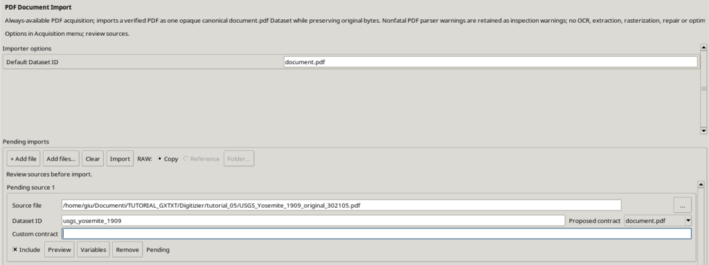
The starting point is a historical topographic map published by the United States Geological Survey (USGS), covering the Yosemite quadrangle, dated 1909 and subsequently reprinted. The map gives elevations in feet and has a 100 ft contour interval. It serves two purposes in this study: it provides a real example of data acquisition from an old document, and it contains recognizable elevation contours suitable for assisted digitization.

It should not, however, be assigned modern levels of precision. The printed documentation also includes a historical note indicating that elevations were subsequently found to be 85 ft too high. In this experiment we retained the elevations printed on the map, without silently applying any altitude correction. The orientation and geometry of a scan can also be distorted: the results therefore use a local Cartesian coordinate system, not geographic or UTM coordinates assigned without supporting georeferencing data.

From image pixels to metric coordinates

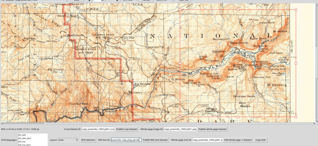
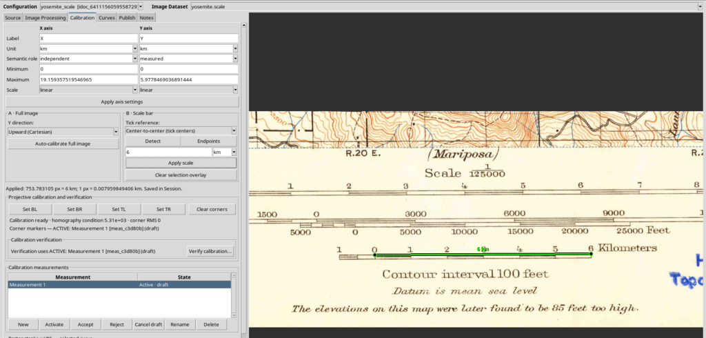
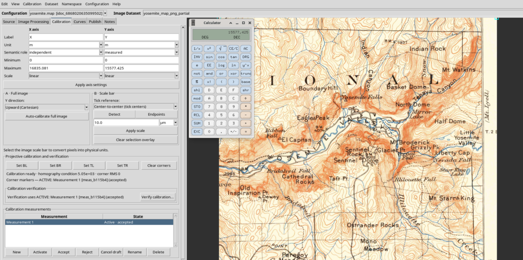
We worked with a raster image extracted from the original PDF at 400 DPI, selecting two separate regions: one containing the terrain to be studied and one containing the scale bar. Keeping the metric reference separate from the study area makes the calibration easier to check.

The essential step is to associate a known distance on the scale bar with a measured distance in pixels. In our case, a 6 km segment corresponds to approximately 753.78 pixels, giving a scale factor close to 7.96 m/pixel. We then used this factor to calibrate the terrain region, with both X and Y axes expressed in metres.

It is not necessary to straighten a scan artificially to obtain a useful demonstration. Here we retained the document’s original geometry, using the scale-bar line as a reference. Nevertheless, the decision must be appropriate for the accuracy required: a local scale calibration does not automatically remove rotation, anisotropic distortions, or cartographic errors.

Digitizing contour lines, not simply drawing lines

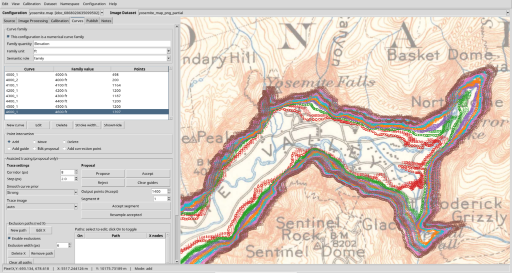
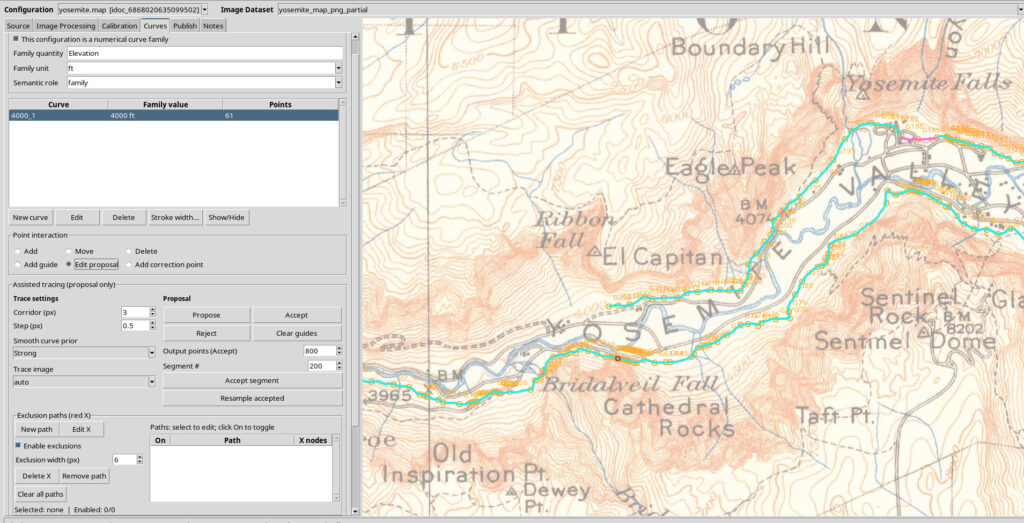
In the GX-TXT Curve Digitalizer, each curve consists of an ordered sequence of points. The assisted tracing feature can follow a recognizable line in the image and allows corrections before acceptance. Visual inspection remains essential with an old map: lettering, rivers, roads, faded areas, and closely spaced lines can confuse automatic recognition.

We configured a numerical curve family with the quantity Elevation and unit ft. The published elevation levels are 4,000, 4,100, 4,200, 4,300, 4,400, 4,500, and 4,600 ft. Two separate traces were digitized at 4,000 ft, giving us eight curves but only seven elevation levels. This structure does not require exactly one curve per elevation, nor a fixed number of points per curve.

The published Dataset

Publication produces a canonical Dataset of type curve_family.table. Each row represents a point, and the information required to reconstruct its parent curve is preserved:

• X and Y: planar coordinates, in metres;
• Curve ID (curve_key): the stable identifier of the trace to which the point belongs;
• Point order (point_order): the point’s position along its curve;
• Family parameter: the elevation of the trace, in feet.

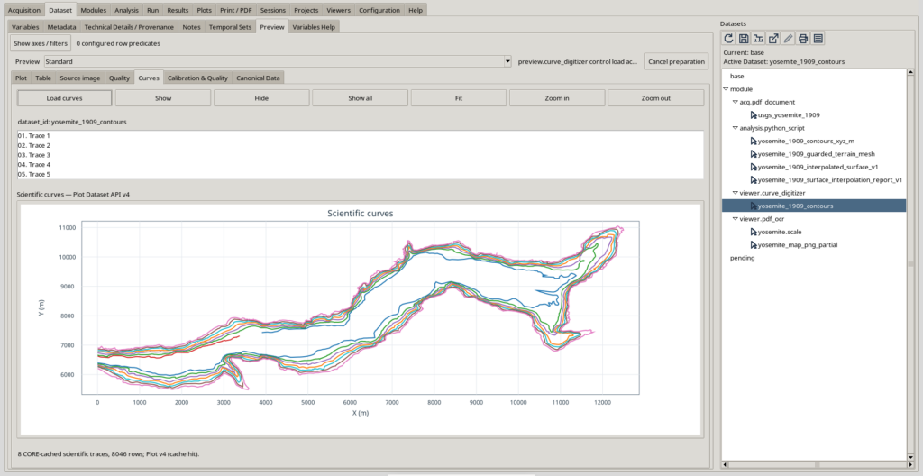
The Dataset used for interpolation is named yosemite_1909_contours and contains 8,046 points. A single Dataset can therefore hold several separate contour lines; there is no need to publish a different Dataset for every curve.

Before building the 3D reconstruction, it is advisable to use the Preview to identify anomalous jumps and straight-line connections that do not follow the map. Points can be in the correct numerical order while their geometry is still wrong: inspecting the graph is an additional scientific check, not merely a cosmetic step.

Why reconstructing a surface is not automatic

A contour line assigns an elevation to points along a line. To build a three-dimensional surface, we must also estimate the elevation between the lines. Using X and Y for the planar coordinates, the desired result is a function:

\[ Z=f(X,Y) \]

This representation is suitable for a conventional single-valued elevation model. It has an important consequence: two different elevations cannot coexist at the same XY point. If digitized contours with different elevations intersect, at least some of the constraints are incompatible with a surface of this kind.

Such crossings may arise from inaccurately placed points, closely spaced segments, errors in the map, ambiguous passages, or an attempt to represent inherently more complex natural geometry as a single-valued surface. Scientific software should not automatically turn these cases into suspended walls or arbitrarily decide which line is correct.

The approach adopted here is to preserve the original Dataset in its entirety, identify problematic regions, and use surrounding observations to reconstruct an interpolated surface wherever possible. The result is a derived model, not a certified correction to the historical document.

---

Python scripts: a reusable workflow

One of the most interesting aspects of this experiment is that the interpolation is not a special function written solely for Yosemite. It is implemented as a Python script executed in Python Script Workspace, which reads a Dataset published by Curve Digitalizer and calls public GX-TXT APIs through Script Bridge.

For readers who want to reproduce or adapt the procedure, three files are central to the workflow:

Script	Purpose	Output
04_interpolate_yosemite_surface_bridge.py	Reads contours, detects conflicts, interpolates the surface, and assesses quality	HDF5 surface Dataset + text report Dataset
05_plot_interpolated_surface_v4.py	Creates two surface plots using Plot Dataset API v4	Elevation plot and distance-to-contour plot
06_finalize_yosemite_plot_v4_scenes.py	Configures the presentation and makes the 3D scenes persistent	Two Native3D representations associated with the plots

The leading numbers are part of the working filenames; they do not represent mandatory chapters in a series of guides. The order of these three scripts does, however, matter when running the complete workflow: first publish the surface, then create the plots, and finally configure the scenes.

All the Python scripts produced during this tutorial are available for download in the Resources section.

Can the main script handle any number of curves?

The number of curves is not fixed at eight. The script reads the Dataset rows and groups them using curve_key. It can therefore work with four, ten, twenty, or more traces, provided that the data requirements and configured computational limits are respected.

More specifically:

• there must be at least two curves at two distinct elevations;
• each curve must contain at least two points in a consistent order;
• different elevations may have different numbers of segments and points;
• two or more curves may share the same elevation;
• the X/Y coordinates must already be calibrated in metres, and the curve family’s elevation parameter must be expressed in feet, as required by the current script.

The script does not identify columns by counting their positions in a CSV file: it uses the semantic roles published in GX-TXT metadata. It can therefore read different sets of curves with the same canonical structure without knowing their IDs in advance. This does not mean that it works unchanged with any numerical table or with different units.

Which APIs actually perform the calculations?

Python handles observation management, grouping, array preparation, and local geometric checks. The core numerical operations are delegated to the framework:

Operation	GX-TXT public API
Reading Datasets and metadata	CANONICAL_DATASET_API_v2, DATASET_METADATA_API_v1, DATASET_VARIABLE_SCHEMA_API_v3
Resampling individual contour lines	NUMERIC_API_v1.interpolate
Two-dimensional interpolation of scattered points	NUMERIC_API_v1.foundation — scattered / interpolate
Grid smoothing filter	NUMERIC_API_v1.linear_matrix
Distance from constraint points	NUMERIC_API_v1.foundation — geometry / kdtree_query
Comparison between the model and observations	NUMERIC_API_v1.foundation — grid / sample and NUMERIC_API_v1.residual_metrics
Surface slope	NUMERIC_API_v1.foundation — calculus / gradient_grid
Publishing the numerical field and report	DATASET_PUBLICATION_API_v2, DATASET_FILE_PUBLICATION_API_v1
Plots and three-dimensional scenes	PLOT_DATASET_API_v4

Checks for intersections between contour segments and some local masks are still implemented using Python/NumPy and scipy.spatial.cKDTree, because we did not use a single public vectorized framework API capable of performing this entire topological analysis. This distinction matters: the script takes advantage of the available numerical APIs, but does not claim that every geometric operation is delegated to GX-TXT.

This architecture is also useful for exploring the framework itself: researchers can identify exactly which operations GX-TXT exposes to scripts, which calculations are executed through the Bridge, and which still require application-specific logic.

Using the scripts in Python Script Workspace

The procedure below describes the reproducible workflow through the graphical interface. In our experiment, the original execution was started programmatically through the public Script Job API, with the Session explicitly specified; this particular launch method is not required to reproduce the results. Users can employ the standard GX-TXT Script Runner.

Preparing the data

Open a GX-TXT Session and publish a numerical curve family from Curve Digitalizer, with X/Y coordinates in metres and elevations in ft. Check the Preview and note the actual Dataset ID: in our example, yosemite_1909_contours.

It is useful to save or duplicate the Session before trying alternative processing methods. This keeps the original Dataset, different interpolation experiments, and final results separate.

Importing and registering the script

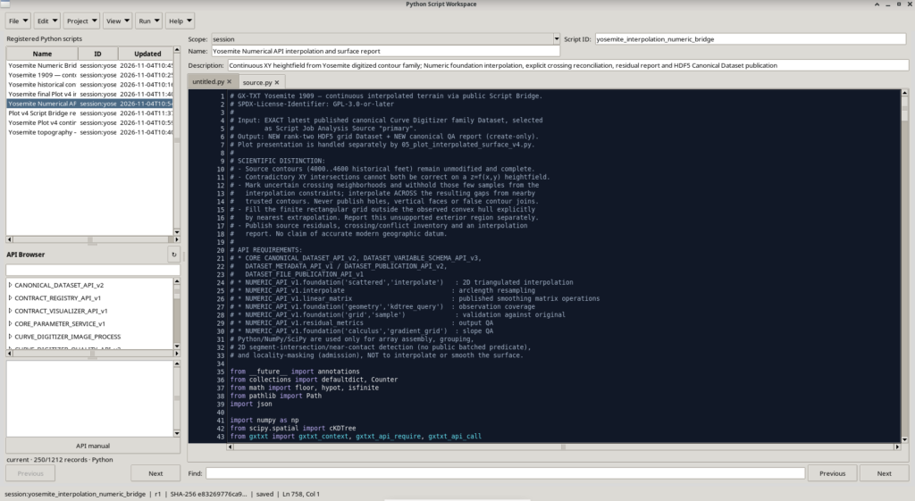
Open Viewers → Python Script Workspace. The Workspace supports importing UTF-8 Python source files through File → Import .py (Ctrl+O), as well as creating new scripts and editing their source code.

1. Import 04_interpolate_yosemite_surface_bridge.py, or paste its contents into a new Python script.
2. Set Scope = Session to keep it in the experiment’s Session, and assign a unique ID. In our example, the registered script ID is yosemite_interpolation_numeric_bridge, with the display name Yosemite Numerical API interpolation and surface report.
3. Check the required APIs and save the script. The Registry records the source revision and hash.
4. Check the value of the INPUT constant in the source: it must match the Dataset that was actually published.

Importing a file does not execute it. The source must be saved and then launched explicitly after reviewing the scientific inputs.

Selecting the input and starting the Job

In the Python Script Workspace Run menu, choose Open Script Runner. The Runner allows you to add an input Dataset and bind it to a semantic alias. For this script, the required alias is exactly primary, and the associated Dataset must match the INPUT constant.

Check the Session, Script ID and revision, source Dataset, Python prerequisites, and available APIs. Use the Runner’s validation function before clicking Run Job. The script performs an additional initial check: if the selected source differs from the expected one, or the required units and semantic roles are missing, it stops rather than publishing an ambiguous Dataset.

This procedure requires a Python environment with NumPy and SciPy, as well as the gxtxt client supplied by the GX-TXT execution environment. It is not intended to run as an ordinary python script.py command outside the framework: in that case, the Session context and public Script Bridge APIs would be unavailable.

Checking that the results have been published

When the Job finishes, the Session should contain two new Datasets:

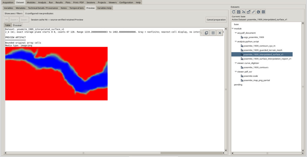
• yosemite_1909_interpolated_surface_v1: the interpolated surface on a regular grid, stored in HDF5;
• yosemite_1909_surface_interpolation_report_v1: the text report containing the method, parameters, topological checks, residuals, and API calls.

The surface contains not only the z_m variable, but also distance_to_contour_m, slope_rise_over_run, outside_hull, and near_conflicting_contours. These fields help identify where the model is less constrained by observations.

The HDF5 grid should not be confused with a simple table of points: z_m is a two-dimensional variable associated with the X and Y axes.

Creating Plot v4 outputs and Native3D scenes

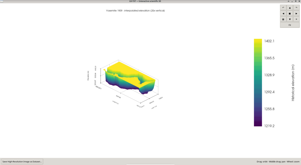
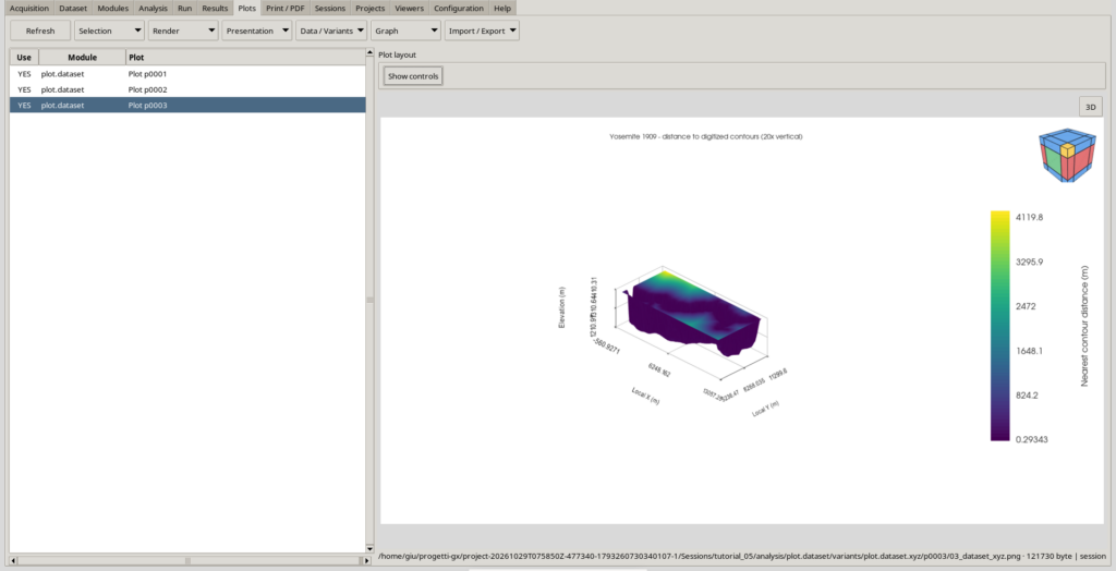
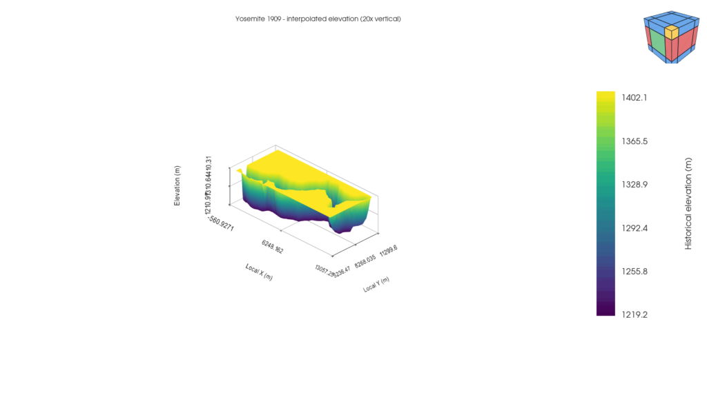
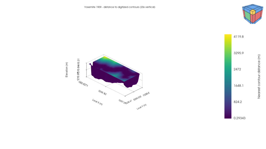
Once the HDF5 Dataset has been published, use 05_plot_interpolated_surface_v4.py in Python Script Workspace, selecting the surface Dataset (rather than the original contours) as the primary input. The script prepares two Plot Dataset v4 representations:

1. Elevation: the z_m values determine the geometry and colouring of the surface.
2. Distance to contour: the geometry remains unchanged, but the colour represents distance_to_contour_m, the planar distance to the nearest digitized constraint points.

Open the plots in GX-TXT and inspect them in the 3D viewer. The file 06_finalize_yosemite_plot_v4_scenes.py can configure the presentation and persistence of the representations programmatically, but it requires particular care with the Variant IDs: in our example Session they were p0002 and p0003, whereas they may differ in a new Session. Read these IDs from the output of the second script and update the references in the third. Do not attempt to force access to the Workspace database while another instance is using it.

For the final presentation, we used an explicitly declared 20× vertical exaggeration to make the terrain profile easier to read. It does not change the stored elevations, but it should be mentioned in the caption to prevent misinterpretation.

---

Adapting the script to another map

The most interesting application is not reproducing the same Yosemite numbers, but transferring the method to other maps or newly digitized contours. The usual changes are concentrated in a few constants and parameters near the beginning of the main script.

Choosing new IDs without overwriting previous work

Near the beginning of 04_interpolate_yosemite_surface_bridge.py, you will find:

INPUT = "yosemite_1909_contours"
OUTPUT = "yosemite_1909_interpolated_surface_v1"
REPORT_DATASET = "yosemite_1909_surface_interpolation_report_v1"

For a new map, set INPUT to the ID of the canonical contour Dataset, and choose two new, unused IDs for OUTPUT and REPORT_DATASET. Publication uses create-only mode: it does not automatically replace an existing Dataset. This is an intentional safeguard against accidental overwriting.

If you change the surface Dataset name, also update DATASET_ID in 05_plot_interpolated_surface_v4.py and DATASET in 06_finalize_yosemite_plot_v4_scenes.py. The Plot Variant IDs used by the final script must then be adapted to those created in the new Session.

Example: to compare two configurations using the same map, you can use the same input data but distinct output IDs, such as terrain_surface_test_a and terrain_surface_test_b, each with its own report. You can then check whether different settings improve the result without losing previous outputs.

Parameters worth understanding

The CFG dictionary in the main script contains the operating parameters. There is no need to rewrite the algorithms to perform a controlled comparison.

Parameter	Value used	What it controls	How to interpret a change
resample_step_m	34 m	Approximate spacing between resampled constraints along the contours	Smaller values add samples and computational work; they do not add original cartographic information
conflict_guard_radius_m	44 m	Neighbourhood around elevation conflicts excluded from estimation constraints	Increasing the radius makes the local reconstruction more conservative, but leaves a larger area to interpolation
close_contact_threshold_m	4 m	Threshold for flagging very close contours at different elevations as problematic	This is a geometric tolerance, not a direct measure of map uncertainty
near_contact_warning_m	16 m	Threshold for reporting close approaches	Produces diagnostic warnings; it does not automatically remove all points within this distance
grid_pitch_m	85 m	Requested grid spacing	Smaller spacing produces more nodes and finer visual detail, but no new measured data
minimum_grid_size / maximum_grid_size	35 / 205	Limits on the number of nodes in each direction	Actual spacing may differ from the requested value to satisfy these limits
smoothing_kernel	[0.16, 0.68, 0.16]	Strength of the smoothing filter along both axes	Use a symmetric, non-negative three-element kernel; giving more weight to neighbours generally smooths the terrain more strongly
confidence_nearest_distance_m	250 m	Distance beyond which a node is flagged as poorly covered	This is a reporting indicator, not a threshold that removes grid cells
maximum_source_rows	100,000	Administrative limit on input points	Increasing it does not automatically guarantee sufficient time or memory

As a starting point, the most sensible approach is to retain the tested parameters and change just one value at a time. Every variant should have new publication IDs and its own report, so that the resulting surface, residuals, and extrapolated area can be compared.

The filter uses a symmetric kernel along both axes, so it is advisable to use a three-element vector of the form [a, b, a], with non-negative weights summing to 1. The current implementation derives both side coefficients from the first element of the vector; changing only the third element will therefore not have the effect you might expect. For more complex experiments, review the matrix-building function deliberately rather than changing the vector at random.

What if the map uses metres instead of feet?

The tested version expects elevations in ft and applies the exact conversion factor:

\[ 1\,\mathrm{ft} = 0.3048\,\mathrm{m} \]

This requirement is also checked against the metadata. To process elevations originally given in metres, changing the Dataset name is not enough: you must consistently adapt the unit check in read_source(), the FT_TO_M conversion factor, variable names, and published metadata. The same applies to maps whose X/Y coordinates are expressed in kilometres or other units.

These changes are relatively limited, but they must be documented and tested. A Dataset expressed in metres but interpreted as feet would produce a formally valid yet scientifically incorrect surface.

What if there are many more contours?

You do not need to enter the number of curves in a constant: the script automatically discovers the Curve IDs and elevation levels present in the Dataset. You can digitize multiple traces at the same elevation or add new levels, while preserving each trace’s curve_key and point order.

Adding more curves does not eliminate topological problems; in fact, it may increase the number of intersections to be investigated. Check the report after every new publication, including the number of nodes retained after excluding conflicting regions. The configured limits on source points, geometric comparisons, and grid dimensions also remain in effect.

A common mistake: confusing higher resolution with greater accuracy

Reducing grid_pitch_m from 85 to 20 metres produces a denser grid, not a better scan or new terrain observations. Many of the resulting nodes would still be estimated from the same digitized traces. Likewise, resampling contours much more finely than the source map’s resolution cannot recover details that the map does not contain.

Quality depends primarily on elevation-data coverage, contour correctness, calibration, and the suitability of the chosen model. Numerical settings can make the result more stable and easier to interpret, but they cannot replace missing observations.

The interpolation report: what really matters

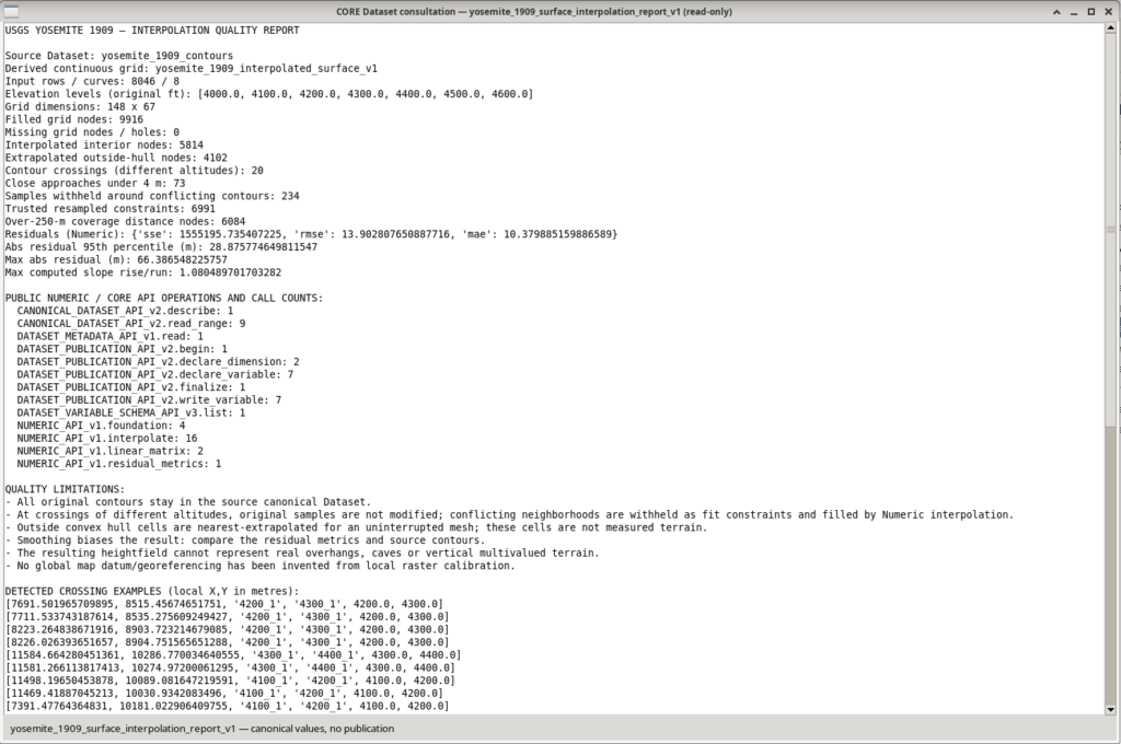
The script does more than generate an image: it records the choices made and provides indicators for assessing the result.

Yosemite experiment indicator	Value
Original curves	8, at 7 elevations
Digitized points in the source Dataset	8,046
XY crossings between contours at different elevations	20
Very close approaches, within 4 m	73
Candidate resampled points	7,225
Points locally excluded as constraints because of conflicts	234
Effective points used for interpolation	6,991
Final grid	148 × 67, or 9,916 nodes
Nodes inside the convex hull, interpolated	5,814
Nodes outside the hull, extrapolated using nearest	4,102 (41.4%)
Nodes without a value (holes)	0
Nodes more than 250 m from the nearest constraint	6,084
RMSE relative to the original points	13.90 m
95th percentile of absolute error at the original points	28.88 m
Maximum absolute error at the original points	66.39 m

The most important result to interpret is coverage: about 41.4% of the rectangular grid nodes lie outside the convex hull of the available constraints. These nodes were assigned values using nearest-neighbour extrapolation. This makes it possible to display a continuous surface without gaps, but it can create extensive flat regions near the boundaries. It does not mean the historical terrain was actually flat.

The value RMSE = 13.90 m also needs careful interpretation: it compares the computed surface with the original contour points. It is a residual relative to the data used in this experiment, not an independent predictive error or an absolute uncertainty in the true terrain elevation. It does not include geodetic validation of the map, a complete estimate of digitization errors, or validation against an external elevation model.

Where contours at different elevations are incompatible, the model does not secretly choose which line to correct. In our experiment, 234 resampled constraints were temporarily excluded from the estimate near conflicts. The original curves remained intact in their canonical Dataset. The report also lists example coordinates and pairs of problematic contours.

How to interpret the two 3D images

The elevation plot answers the question: what continuous surface results from applying the chosen method to the digitized contours? The colour scale shows elevations in metres. Apparent terraces or steep walls near the coverage boundaries should be compared with the second image, rather than immediately interpreted as real geomorphological features.

The distance-to-contour plot answers a different question: where is the model close to digitized points, and where is it farther away? It is not a probabilistic uncertainty map; it is a geometric indicator of observational support. The most distant regions are those where additional contours might improve the model the most.

What to check when changing the Dataset

Before considering a reconstruction of a different map satisfactory, we suggest four simple, repeatable checks:

1. Calibration and units. Check the known distance, X/Y units, and elevation units. Do not assume another map uses the same foot units or map scale.
2. Contour continuity. Inspect the Preview for segments connecting distant areas, off-trace points, overlaps, and unexpected directions.
3. Interpolation report. Compare the number of retained points, crossings, residuals, and extrapolated fraction. A continuous model is not automatically a reliable model.
4. Plots alongside the original data. Check that the most prominent model features are compatible with the observed contours; do not rely on the 3D rendering alone.

To improve reliability, the best investment is often not a different algorithm, but digitizing additional contours in poorly covered regions, keeping curve identities, elevations, and point order consistent. The script can then be run again on a newly published Dataset, using new output IDs and comparing the reports.

A general method, with explicitly stated limitations

This experiment shows how to connect three activities that are often kept separate: scientific digitization of a document, numerical processing through public APIs, and publication of inspectable results and persistent 3D representations within the same GX-TXT Session.

With the necessary adaptations, the procedure can be applied to other historical maps, elevation profiles, or datasets represented by families of curves with assigned elevations. It does not replace a georeferenced DEM or a modern topographic survey: it produces a verifiable interpretive reconstruction, accompanied by an explicit description of its assumptions and less reliable regions.

Making the script public does more than show how an image was generated. It allows readers to add more curves, change grid density, compare different strategies, and document the results without having to rewrite the analysis process from scratch.

---

Resources for reproducing the experiment

Download Python scripts:

Map used:

Yosemite Quadrangle, 1909 edition, 1951 reprint, identifier 302105

Software used in this experiment: GX-TXT DEV112, Curve Digitalizer, Python Script Workspace, NUMERIC_API_v1, Canonical Dataset API, Plot Dataset API v4, and Native3D.