

GX-TXT Curve Digitalizer: From a TLC Photograph to Retention Factors with Python
Thin-layer chromatography, or TLC, is a simple, versatile technique for separating and comparing the components of a mixture. In a typical experiment, the spots developed on the plate are examined, the application baseline and the distance traveled by the solvent front are identified, and the distances required to calculate the retention factor, denoted by \(R_f\), are measured.
In this experiment, we use GX-TXT Curve Digitalizer to turn a real photograph of a TLC plate into a Dataset of coordinates. Then, using a Python script executed inside GX-TXT, we calculate the geometric centroids of the annotated regions, obtain five \(R_f\) values, publish the results as a scientific table, and visualize them in the CORE Scientific Dataset Viewer.
We will not use an artificial photograph or a table of invented values. Our starting point is an existing image bearing annotations made by the person who performed the experiment. This makes the example particularly useful for teaching, but it also requires us to distinguish what can actually be measured from the photograph from what would require independent chemical verification.
The TLC photograph and the materials required
The photograph comes from Amino acids TLC with English translation, published on Wikimedia Commons by Dvnyn as an adaptation of material attributed to TheFatDrummer. The original work is available under the Creative Commons CC BY-SA 4.0 license.

The full source image contains both a photograph of the TLC plate and an explanatory diagram. For GX-TXT, we prepared a crop containing only the photograph, without changing its colors or reconstructing any spots. The image used in the experiment is 1500 × 2010 pixels. We provide the ready-to-import photograph so readers do not need any cropping scripts or preparation procedure.
Download the photograph used in this experiment:
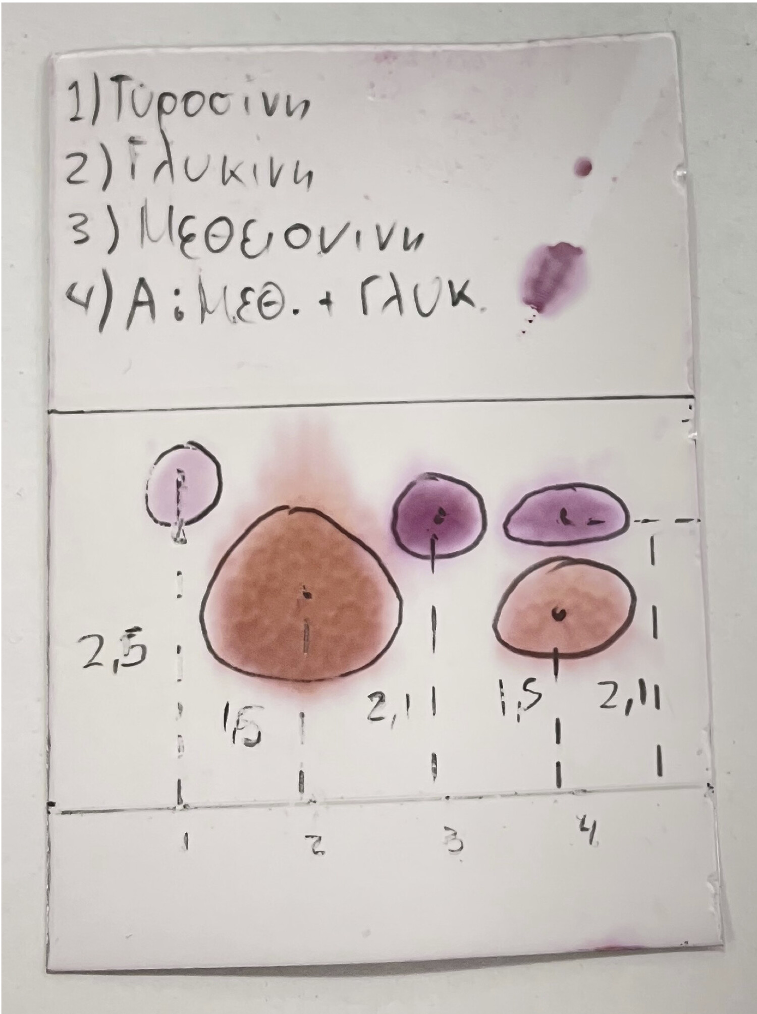
To view the complete original image and its attribution, visit the original page on Wikimedia Commons, which also provides a direct download of the original PNG.

Four lanes are labeled in the photograph: three reference substances identified by the source as tyrosine, glycine, and methionine, and a fourth lane containing a mixture attributed to glycine and methionine. The handwritten labels and marker outlines are already part of the source image. They help us build a reproducible exercise, but they do not constitute an independent analytical identification.
Import and calibrate the plate, not the entire photograph
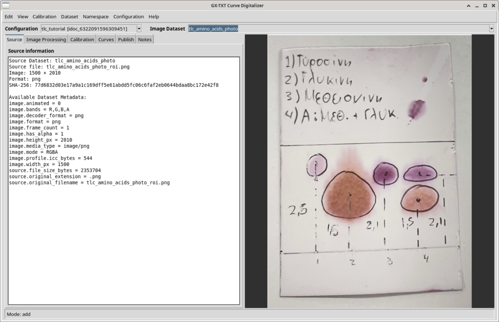
The first step is to import the image into a GX-TXT Session as an Image Dataset and open it in Curve Digitalizer. The source photograph does not contain an independent physical length reference from which millimeters or centimeters can be established reliably. This does not prevent our analysis, because \(R_f\) is dimensionless.
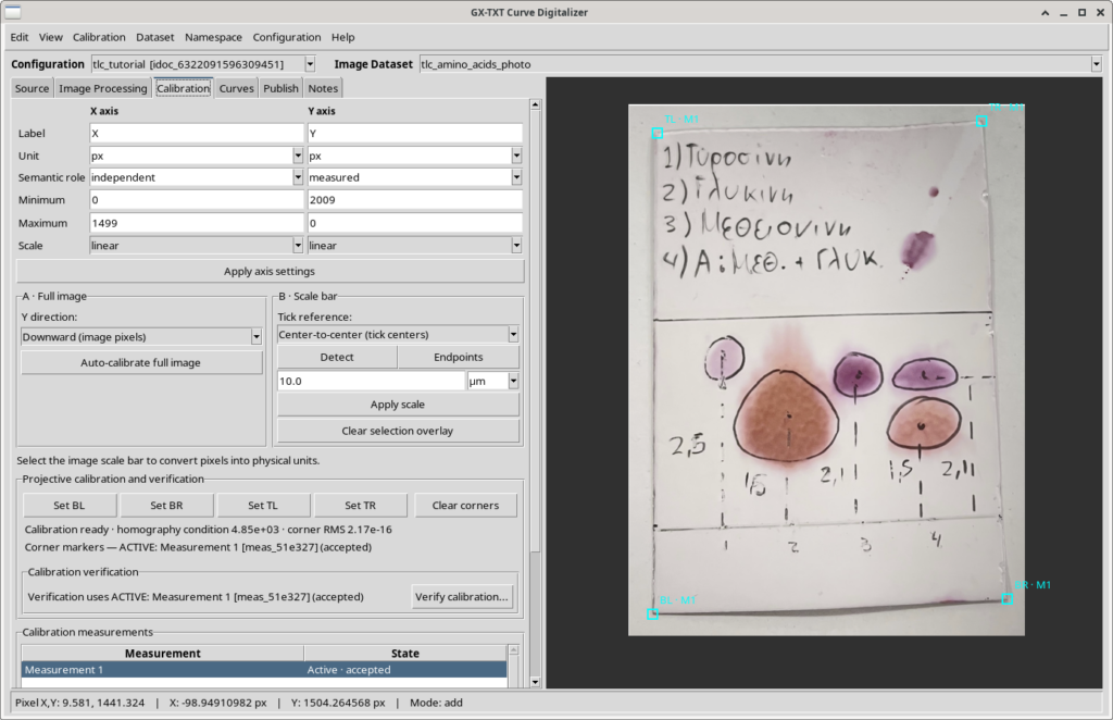
What matters is that the coordinates accurately represent the plane of the TLC plate, which was photographed with some perspective distortion. We therefore used a manual four-point projective calibration, selecting the actual plate corners rather than the corners of the PNG or the background sheet. The references in the Calibration panel are:
- BL (Bottom Left): the lower-left corner of the plate;
- BR (Bottom Right): the lower-right corner;
- TL (Top Left): the upper-left corner;
- TR (Top Right): the upper-right corner.
GX-TXT computes a projective transformation, or homography, that expresses all digitized positions within one coordinate system. In our experiment, both axes remain linear and use the nominal unit px. These are coordinates of the projectively rectified plate, not certified physical distances. The calibration was checked and accepted before the curves were digitized.
Projective rectification does not necessarily remove camera-lens distortion or correct physical deformation of the plate. Nevertheless, it is more appropriate here than automatic calibration against the four corners of the entire image.
Digitize the application baseline and the solvent front
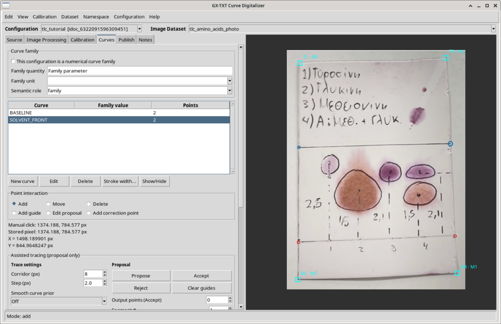
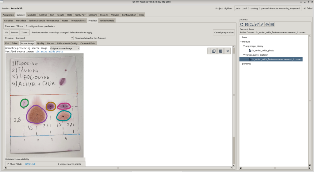
Two references are required to calculate the retention factor. In the Curves tab, we create two independent curves, each defined by two points:
BASELINE, representing the application line near the lower part of the plate;SOLVENT_FRONT, representing the upper line interpreted as the position reached by the solvent.
It is useful to define these references as line segments rather than assuming they have a constant vertical coordinate. This allows the script to compute migration distances while accounting for the orientation of each line.
The interpretation of the upper line as the solvent front is based on the photograph and its annotations. For an independent analytical measurement, this interpretation would need confirmation from the original experimental documentation.
The five spots: digitizing annotated regions
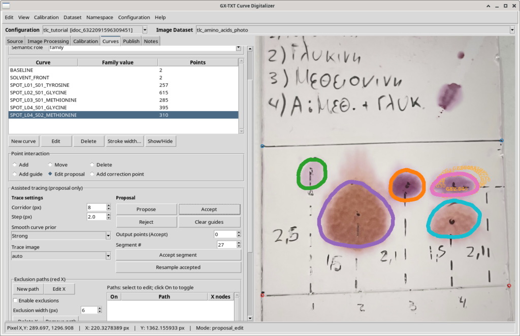
In the photograph, the chemist drew outlines around the spots with a marker. We chose to digitize precisely those boundaries rather than invent a color threshold or simulate automatic image segmentation. This makes the procedure reproducible: readers can trace the same marked regions on the image.
The five curves are named as follows:
| Lane | Curve name | Region identified in the photograph |
|---|---|---|
| 1 | SPOT_L01_S01_TYROSINE | Tyrosine |
| 2 | SPOT_L02_S01_GLYCINE | Glycine |
| 3 | SPOT_L03_S01_METHIONINE | Methionine |
| 4 | SPOT_L04_S01_GLYCINE | Lower spot in the mixture |
| 4 | SPOT_L04_S02_METHIONINE | Upper spot in the mixture |
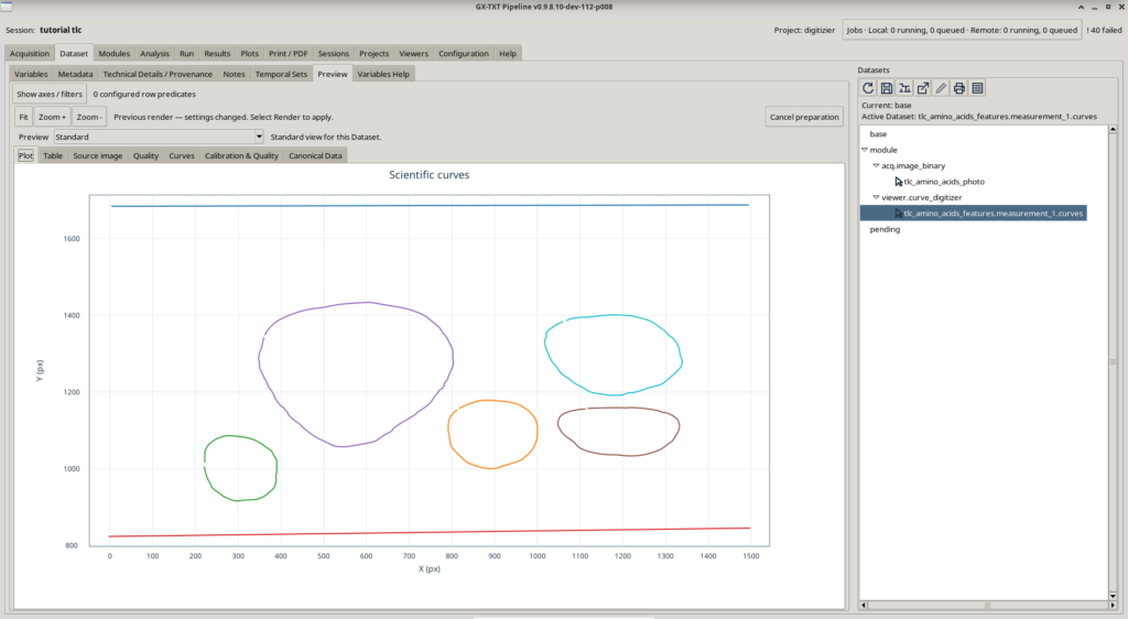
The curves are kept in independent curves mode, rather than being treated as a numerical curve family. Each outline consists of an ordered sequence of points. We used detailed digitization to preserve the irregularities in the original hand-marked shapes.
Tyrosine requires a qualification: its stain is very faint. Its outline was digitized because it was marked on the original photograph, not because the actual boundary of the colored region could be determined with the same confidence as for the other spots. Accordingly, the resulting measurements describe the marker-defined region.
Publish the coordinates as a GX-TXT Dataset
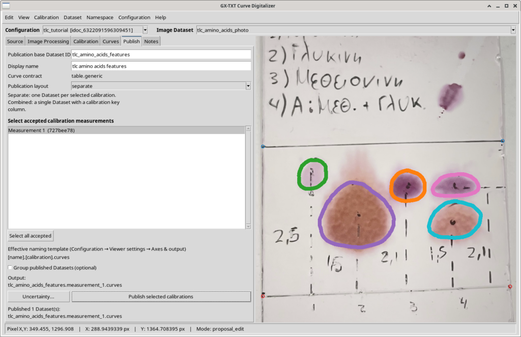
Once digitization is complete, the Publish tab allows the coordinates to be saved as a canonical Dataset. For this experiment, we selected an accepted calibration measurement, chose the separate-per-calibration publication layout, and retained the table.generic contract, which is suitable for independent curves.
The actual publication contains seven curves—the two reference segments and the five spot regions—with a total of 1,866 points. Each row preserves scientific coordinates, original image coordinates, curve identity, and point order. These fields allow the script to reconstruct the outlines rather than merely reading an unordered table of X and Y values.
GX-TXT may append a suffix identifying the selected calibration. In this experiment, for example, the source Dataset was published as tlc_amino_acids_features.measurement_1.curves. There is no need to enter this identifier into the Python code: we select it as an input Dataset when running the script.
From spot outlines to retention factors
The retention factor of a TLC spot is defined as the distance traveled by the compound divided by the distance traveled by the solvent front, both measured from the application baseline:
\[ R_f = \frac{d_{\mathrm{spot}}}{d_{\mathrm{front}}} \]
No conversion to centimeters is necessary provided both distances are defined in the same coordinate system.
Our script does not choose an arbitrary point inside a spot. It treats each outline as a polygon and computes its geometric centroid—the center of area of the enclosed region:
\[ \mathbf{c}=\frac{1}{A}\iint_{\Omega}(x,y)\,\mathrm{d}A \]
This definition is useful when regions are asymmetric or irregular: choosing a single central point by eye would be more subjective. The region is closed geometrically by joining the final point to the first one. The script also checks the size of any remaining closure gap.
To determine migration distances, the program calculates the normal direction to BASELINE and evaluates the solvent front at the position corresponding to each spot. This is more general than merely subtracting two Y coordinates: it also works when the reference lines are not perfectly horizontal.
The calculated area and perimeter describe the annotated polygon, not a physical measurement in square millimeters or an assessment of the quantity of compound present. The program produces several geometric quantities, but the main chromatographic result remains \(R_f\).
The Python script: how to use it
The main program is tlc_rf_table_generic_csv.py. It is designed to work with other TLC photographs as well: it is not tied to the name of our Dataset and is not limited to the five spots in this example.
#!/usr/bin/env python3
# SPDX-License-Identifier: GPL-3.0-or-later
"""Generic TLC Rf table Dataset from a Curve Digitalizer canonical Dataset.

Use Python Script Workspace -> Run -> Open Script Runner, and choose the
published Curve Digitalizer Dataset as Analysis Source with alias 'primary'.

No source Dataset ID or technical input column name is hardcoded.
The actual Curve Digitalizer roles and Variable IDs are obtained using public
Dataset Metadata API v1 and Variable Schema API v3 through the Script Bridge.
The public Curve Digitizer Dataset Schema host API is not Script-bridged in
the currently installed framework, so it cannot be called from Python.

Curve *labels* distinguish BASELINE, SOLVENT_FRONT and SPOT_Lnn_Snn_*;
edit the three conventions below if a different naming scheme was used.
The ROI contours are annotations by an operator, not automatic segmentation.
Only one canonical table.generic CSV Dataset is published. A separate Markdown
note is prepared in the Job output for attachment via GX-TXT Dataset Notes UI;
Python Script Bridge does not expose the host-only Dataset Notes writer.
"""

from __future__ import annotations

from collections import defaultdict
from hashlib import sha256
from math import dist, hypot, isfinite
from pathlib import Path
import json
import re

from gxtxt import gxtxt_api_call, gxtxt_api_require, gxtxt_context

SOURCE_ALIAS = "primary"
BASELINE_LABEL = "BASELINE"
FRONT_LABEL = "SOLVENT_FRONT"
SPOT_LABEL_PATTERN = r"^SPOT_L(\d{1,3})_S(\d{1,3})(?:_[A-Z0-9_]+)?$"
RESULT_VERSION = "v2"          # Choose v2, v3 ... to publish another analysis.
MAX_SOURCE_ROWS = 100000
MAX_GAP_FRACTION = 0.10        # Safety check for obviously open polygons.
SPOT_PATTERN = re.compile(SPOT_LABEL_PATTERN)

REQUIRED_APIS = [
    "CANONICAL_DATASET_API_v2@2",
    "DATASET_METADATA_API_v1@1",
    "DATASET_VARIABLE_SCHEMA_API_v3@3",
    "DATASET_PUBLICATION_API_v2@2",
]


def api(owner, operation, args):
    return gxtxt_api_call(owner, operation, args)


def selected_source(ctx):
    inputs = ctx.get("inputs", {}) or {}
    source = (inputs.get(SOURCE_ALIAS, {}) or {}).get("dataset_id", "")
    source = str(source).strip()
    if not source:
        raise RuntimeError(
            "In Open Script Runner, add a Dataset input with alias 'primary'.")
    return source


def output_names(source):
    stem = re.sub(r"[^a-z0-9_]+", "_", source.lower()).strip("_")
    if len(stem) > 66:
        stem = stem[:54].rstrip("_") + "_" + sha256(source.encode()).hexdigest()[:9]
    if not stem or not re.fullmatch(r"v[1-9][0-9]*", RESULT_VERSION):
        raise RuntimeError("Invalid source identity or RESULT_VERSION")
    return stem + "_rf_" + RESULT_VERSION


def _column(block, variable_id):
    source = block[variable_id]["values"]
    if hasattr(source, "reshape"):
        return source.reshape(-1).tolist()
    result = []
    for value in source:
        if isinstance(value, (list, tuple)):
            if len(value) != 1:
                raise RuntimeError("Non-rank-one canonical input column")
            value = value[0]
        result.append(value)
    return result


def read_digitizer_source(dataset_id):
    """Resolve the producer's role manifest, not CSV headers or fixed IDs."""
    md = api("DATASET_METADATA_API_v1", "read", [dataset_id])
    if md.get("curve_digitizer.plugin_id") != "viewer.curve_digitizer":
        raise RuntimeError("The selected Dataset was not published by Curve Digitalizer")
    if md.get("curve_digitizer.curve_mode") != "independent":
        raise RuntimeError("Select a Dataset of independent digitized curves")
    if md.get("curve_digitizer.curve_grouping") != "curve_key":
        raise RuntimeError("Select a single-calibration publication (curve_key grouping)")
    schema_version = str(md.get("curve_digitizer.curve_schema_version", ""))
    if schema_version not in ("1", "2"):
        raise RuntimeError("Unsupported or missing Curve Digitalizer schema version")

    desc = api("CANONICAL_DATASET_API_v2", "describe", [dataset_id])
    if desc.get("contract") != "table.generic":
        raise RuntimeError("Expected Curve Digitalizer table.generic contract")
    rows = int(desc.get("row_count", 0))
    if rows < 7 or rows > MAX_SOURCE_ROWS:
        raise RuntimeError("Unexpected source point count: " + str(rows))

    schema = api("DATASET_VARIABLE_SCHEMA_API_v3", "list", [dataset_id])
    by_id = {str(col["variable_id"]): col for col in schema}
    roles = ("x", "y", "curve_key", "curve_name", "point_order")
    columns = {}
    dimension = str(md.get("curve_digitizer.curve_row_dimension", ""))
    if not dimension:
        raise RuntimeError("Missing Curve Digitalizer row dimension metadata")
    for role in roles:
        key = "curve_digitizer.curve_column." + role
        variable_id = str(md.get(key, "")).strip()
        if not variable_id or variable_id not in by_id:
            raise RuntimeError("Missing producer semantic column role: " + role)
        col = by_id[variable_id]
        if str(col.get("rank")) != "1":
            raise RuntimeError("Non-scalar producer column for role: " + role)
        declared_dimensions = col.get("dimension_ids")
        if isinstance(declared_dimensions, (list, tuple)):
            declared_dimensions = list(declared_dimensions)
        elif isinstance(declared_dimensions, str):
            declared_dimensions = declared_dimensions.replace(";", " ").split()
        else:
            declared_dimensions = []
        if declared_dimensions != [dimension]:
            raise RuntimeError("Producer column dimension mismatch: " + role)
        columns[role] = variable_id
    if len(set(columns.values())) != len(roles):
        raise RuntimeError("Duplicate Variable IDs mapped to different roles")
    xy_unit = str(by_id[columns["x"]].get("unit", ""))
    if not xy_unit or xy_unit != str(by_id[columns["y"]].get("unit", "")):
        raise RuntimeError("X and Y must share a consistent unit")
    if xy_unit not in ("px", "1", "mm", "cm", "m"):
        raise RuntimeError("Review unfamiliar source unit: " + xy_unit)

    curves_by_key = defaultdict(list)
    names_by_key = {}
    wanted = list(dict.fromkeys(columns.values()))
    for start in range(0, rows, 1000):
        count = min(1000, rows - start)
        block = api("CANONICAL_DATASET_API_v2", "read_range",
                    [dataset_id, wanted, start, count])
        data = {role: _column(block, var) for role, var in columns.items()}
        if any(len(v) != count for v in data.values()):
            raise RuntimeError("Canonical read_range returned incomplete data")
        for i in range(count):
            x, y = float(data["x"][i]), float(data["y"][i])
            key = str(data["curve_key"][i]).strip()
            name = str(data["curve_name"][i]).strip().upper()
            order = int(data["point_order"][i])
            if not (isfinite(x) and isfinite(y) and key and name):
                raise RuntimeError("Invalid Curve Digitalizer point")
            if key in names_by_key and name != names_by_key[key]:
                raise RuntimeError("Conflicting labels for one curve key")
            names_by_key[key] = name
            curves_by_key[key].append((order, (x, y)))

    curves = {}
    for key, rows_for_curve in curves_by_key.items():
        rows_for_curve.sort(key=lambda item: item[0])
        if [v[0] for v in rows_for_curve] != list(range(len(rows_for_curve))):
            raise RuntimeError("Inconsistent point_order for curve " + key)
        label = names_by_key[key]
        if label in curves:
            raise RuntimeError("Duplicate curve label: " + label)
        curves[label] = [xy for _, xy in rows_for_curve]
    return curves, xy_unit, rows, columns


def dot(u, v):
    return u[0]*v[0] + u[1]*v[1]


def sub(a, b):
    return a[0]-b[0], a[1]-b[1]


def polygon_centroid(vertices):
    """Shoelace centroid for a closed hand-annotated contour."""
    if len(vertices) < 3:
        raise RuntimeError("Spot contour requires three or more points")
    pts = vertices[:-1] if dist(vertices[0], vertices[-1]) < 1e-8 else vertices
    if len(pts) < 3:
        raise RuntimeError("Degenerate polygon")
    cross_sum = sum_x = sum_y = perimeter = 0.0
    for a, b in zip(pts, pts[1:] + pts[:1]):
        cross = a[0]*b[1] - b[0]*a[1]
        cross_sum += cross
        sum_x += (a[0] + b[0])*cross
        sum_y += (a[1] + b[1])*cross
        perimeter += dist(a, b)
    if abs(cross_sum) < 1e-8 or perimeter < 1e-8:
        raise RuntimeError("Spot has invalid polygon area or perimeter")
    gap = dist(vertices[0], vertices[-1])
    if gap/perimeter > MAX_GAP_FRACTION:
        raise RuntimeError("Contour closure gap exceeds the reviewed limit")
    centroid = (sum_x/(3*cross_sum), sum_y/(3*cross_sum))
    if not all(isfinite(z) for z in centroid):
        raise RuntimeError("Non-finite polygon centroid")
    return centroid, abs(cross_sum)/2, perimeter, gap


def rf_measurements(curves):
    """Measure each ROI by its perpendicular distance along the plate."""
    baseline = curves.get(BASELINE_LABEL)
    front = curves.get(FRONT_LABEL)
    if baseline is None or front is None:
        raise RuntimeError("Missing BASELINE or SOLVENT_FRONT annotated curves")
    if len(baseline) != 2 or len(front) != 2:
        raise RuntimeError("BASELINE and SOLVENT_FRONT need exactly two points each")
    b0, b1 = baseline
    f0, f1 = front
    direction = sub(b1, b0)
    length = hypot(*direction)
    if length <= 1e-9:
        raise RuntimeError("Degenerate baseline segment")
    tangent = direction[0]/length, direction[1]/length
    normal = (-tangent[1], tangent[0])
    midpoint_front = ((f0[0]+f1[0])/2, (f0[1]+f1[1])/2)
    if dot(sub(midpoint_front, b0), normal) < 0:
        normal = (-normal[0], -normal[1])
    front_pos0 = dot(sub(f0, b0), tangent)
    front_delta = dot(sub(f1, f0), tangent)
    if abs(front_delta) < 1e-9:
        raise RuntimeError("Front is transverse to the migration coordinate")
    min_u, max_u = sorted((front_pos0, front_pos0+front_delta))

    observations = []
    for name, points in sorted(curves.items()):
        if name in (BASELINE_LABEL, FRONT_LABEL):
            continue
        match = SPOT_PATTERN.fullmatch(name)
        if match is None:
            raise RuntimeError(
                f"Unknown spot curve label: {name}; change SPOT_LABEL_PATTERN")
        centroid, area, perimeter, gap = polygon_centroid(points)
        u = dot(sub(centroid, b0), tangent)
        if not min_u-1e-6 <= u <= max_u+1e-6:
            raise RuntimeError("Spot lies outside the annotated solvent front: "+name)
        f = (u-front_pos0)/front_delta
        front_here = (f0[0]+f*(f1[0]-f0[0]),
                      f0[1]+f*(f1[1]-f0[1]))
        d_solvent = dot(sub(front_here, b0), normal)
        d_spot = dot(sub(centroid, b0), normal)
        if d_solvent <= 0:
            raise RuntimeError("Nonpositive migration distance: " + name)
        retention = d_spot/d_solvent
        if not 0.0 <= retention <= 1.0:
            raise RuntimeError("Rf outside [0,1]; check source lines: " + name)
        observations.append({
            "name": name,
            "lane": int(match.group(1)),
            "spot_index": int(match.group(2)),
            "centroid_x": centroid[0],
            "centroid_y": centroid[1],
            "distance_spot": d_spot,
            "distance_front": d_solvent,
            "rf": retention,
            "annotated_area": area,
            "annotated_perimeter": perimeter,
            "closure_gap": gap,
            "source_points": len(points),
        })
    if not observations:
        raise RuntimeError("No SPOT_Lnn_Snn curves in selected input Dataset")
    if len({(r["lane"],r["spot_index"]) for r in observations}) != len(observations):
        raise RuntimeError("Duplicate lane and spot identifiers")
    return observations


TABLE_FIELDS = (
    # Stable column IDs, readable labels, internal field, dtype, unit rule.
    ("feature_name", "Digitized feature label", "name", "string", "text"),
    ("lane", "TLC lane", "lane", "int32", "1"),
    ("spot_index", "Spot within lane", "spot_index", "int32", "1"),
    ("rf", "Retention factor (Rf)", "rf", "float64", "1"),
    ("spot_distance", "Spot migration distance (mapped coordinates)",
     "distance_spot", "float64", "unit"),
    ("solvent_distance", "Solvent-front migration distance (mapped coordinates)",
     "distance_front", "float64", "unit"),
    ("centroid_x", "Annotated region centroid X",
     "centroid_x", "float64", "unit"),
    ("centroid_y", "Annotated region centroid Y",
     "centroid_y", "float64", "unit"),
    ("annotated_area", "Annotated region area (mapped coordinates squared)",
     "annotated_area", "float64", "area"),
    ("annotated_perimeter", "Annotated region perimeter",
     "annotated_perimeter", "float64", "unit"),
    ("closure_gap", "Unclosed contour gap",
     "closure_gap", "float64", "unit"),
    ("source_points", "Original digitized points",
     "source_points", "int32", "1"),
)


def _unit_for_field(u, coordinate_unit):
    if u == "text":
        return ""
    if u == "unit":
        return coordinate_unit
    if u == "area":
        return "1" if coordinate_unit == "1" else coordinate_unit + "^2"
    return u


def publish_table_dataset(source, output, unit, measurements, column_roles,
                          original_rows):
    metadata = {
        "processing.kind": "tlc_retention_factor_from_annotated_polygons",
        "processing.input_dataset_id": source,
        "processing.input_coordinate_unit": unit,
        "processing.source_rows": str(original_rows),
        "processing.spot_count": str(len(measurements)),
        "processing.method": "chemist_marker_polygon_centroid",
        "processing.rf_method": "baseline_normal_perpendicular_distance_ratio",
        "processing.geometry": "source_projective_calibration",
        "processing.uncertainty": "not_quantified",
        "processing.spot_identities": "source_labels_only_not_verified",
        "processing.input_column_mapping": json.dumps(
            column_roles, sort_keys=True, ensure_ascii=False),
        "processing.annotation_type": "chemist_drawn_marker_ROI",
        "processing.rf_definition": "spot_distance_divided_by_solvent_distance",
        "processing.coordinate_reference": "projectively_mapped_TLC_plate",
    }
    definition = {
        "dataset_id": output,
        "contract": "table.generic",
        "storage": "csv",
        "producer_version": "2.0.0",
        "replace_owned": False,
        "source_dataset_ids": [source],
        "source_variable_ids": [],
        "source": "GX-TXT Python Script Workspace public Script Bridge",
        "provenance": (
            "TLC geometric centroid and Rf from a published Curve Digitalizer "
            "Dataset; validated producer semantic columns; single canonical table."),
        "structured_metadata": metadata,
    }
    writer = api("DATASET_PUBLICATION_API_v2", "begin", [definition])
    try:
        api("DATASET_PUBLICATION_API_v2", "declare_dimension",
            [writer, "row", 0, {"extendible": True}])
        columns = {}
        for field_id, label, key, dtype, unit_rule in TABLE_FIELDS:
            schema = {
                "dtype": dtype,
                "rank": 1,
                "dimension_ids": "row",
                "coordinate_role": "data",
                "name": field_id,
                "display_label": label,
                "unit": _unit_for_field(unit_rule, unit),
                "semantic_role": "" if dtype == "string" else "derived",
            }
            api("DATASET_PUBLICATION_API_v2", "declare_variable",
                [writer, field_id, schema])
            if dtype == "string":
                vals = [str(item[key]) for item in measurements]
            elif dtype == "int32":
                vals = [int(item[key]) for item in measurements]
            else:
                vals = [float(item[key]) for item in measurements]
            columns[field_id] = vals
        api("DATASET_PUBLICATION_API_v2", "append",
            [writer, "row", columns])
        receipt = api("DATASET_PUBLICATION_API_v2", "finalize", [writer])
        writer = None
        return receipt
    except Exception:
        if writer is not None:
            api("DATASET_PUBLICATION_API_v2", "abort", [writer])
        raise


def prepare_dataset_notes(source, output, unit, columns, source_rows,
                          measurements, ctx):
    # The current Python Script Bridge has NO Dataset Notes API write operation.
    # Do not manufacture a second Dataset or mutate the Session registry.
    # Save reviewable Markdown in the owned Job output directory; attach it in
    # the ordinary Dataset -> Notes editor after verifying the published table.
    root = Path(ctx["output_dir"]).resolve()
    root.mkdir(parents=True, exist_ok=True)
    lines = [
        "# TLC retention factor — scientific notes",
        "",
        "## Provenance",
        "",
        "Source Dataset: " + source,
        "",
        "Result Dataset: " + output,
        "",
        "Original Curve Digitalizer rows: " + str(source_rows),
        "",
        "Coordinate unit in source: " + unit,
        "",
        "The spot regions were **drawn in marker by a chemist** on the "
        "original photograph. We digitized those annotations, not automatically "
        "segmented chemical stain boundaries. Chemical names are source "
        "labels, not independently verified identities.",
        "",
        "## Method",
        "",
        "Each annotated contour was treated as a polygon. Its shoelace "
        "centroid was projected onto the migration direction, defined as the "
        "normal to BASELINE. The solvent front was evaluated at the same "
        "baseline-tangent coordinate. Rf equals spot migration distance "
        "divided by solvent-front migration distance.",
        "",
        "Values are dimensionless; source coordinate units describe a "
        "projectively mapped plate, **not a certified physical mm scale**.",
        "",
        "## Measured spots",
        "",
        "| Source curve name | Lane | Spot | Rf |",
        "|---|---:|---:|---:|",
    ]
    for item in measurements:
        lines.append(
            "| " + str(item["name"]) + " | " +
            str(item["lane"]) + " | " +
            str(item["spot_index"]) + " | " +
            format(item["rf"], ".6f") + " |")
    lines.extend([
        "",
        "## Producer semantic role mappings",
        "",
        "Resolved from the source's Curve Digitalizer metadata and the "
        "public Variable Schema API, not from hardcoded CSV column headers.",
        "",
    ])
    for role, var_id in sorted(columns.items()):
        lines.append("- " + role + ": " + var_id)
    lines.extend([
        "",
        "## Limitations",
        "",
        "- The upper reference line is presumed to be the solvent front; "
        "its identity requires experimental confirmation.",
        "- A manually drawn perimeter may not coincide exactly with the stain.",
        "- The faint tyrosine region is especially sensitive to operator annotation.",
        "- Rf alone cannot establish chemical identity or concentration.",
        "- Lens distortion and nonplanarity are not corrected by a projective mapping.",
        "- Source-coordinate uncertainties and propagated Rf uncertainties "
        "have not been quantified.",
        "",
        "This note can be associated via the GX-TXT Dataset Notes editor. "
        "It is not a second scientific Dataset.",
        "",
    ])
    path = root / "tlc_rf_dataset_notes.md"
    path.write_text("\n".join(lines),
                    encoding="utf-8")
    return path


def main():
    gxtxt_api_require(REQUIRED_APIS)
    ctx = gxtxt_context()
    source = selected_source(ctx)
    output = output_names(source)
    curves, unit, count, columns = read_digitizer_source(source)
    observations = rf_measurements(curves)
    print("TLC_INPUT", source, "rows", count, "curves", len(curves))
    print("TLC_DISCOVERED_ROLES", columns)
    for row in observations:
        print("TLC_RF", row["name"], format(row["rf"], ".6f"))
    notes = prepare_dataset_notes(source, output, unit, columns, count,
                                  observations, ctx)
    print("TLC_DATASET_NOTES_MARKDOWN_READY", str(notes), flush=True)
    receipt = publish_table_dataset(source, output, unit, observations,
                                    columns, count)
    print("TLC_TABLE_DATASET_PUBLISHED", receipt, flush=True)
    print("TLC_NOTE_ATTACHMENT_REQUIRED",
          "Use Dataset -> Notes to associate the Markdown with the new Dataset",
          flush=True)


if __name__ == "__main__":
    main()
To run the analysis:
- Open the Session containing the Dataset published by Curve Digitalizer.
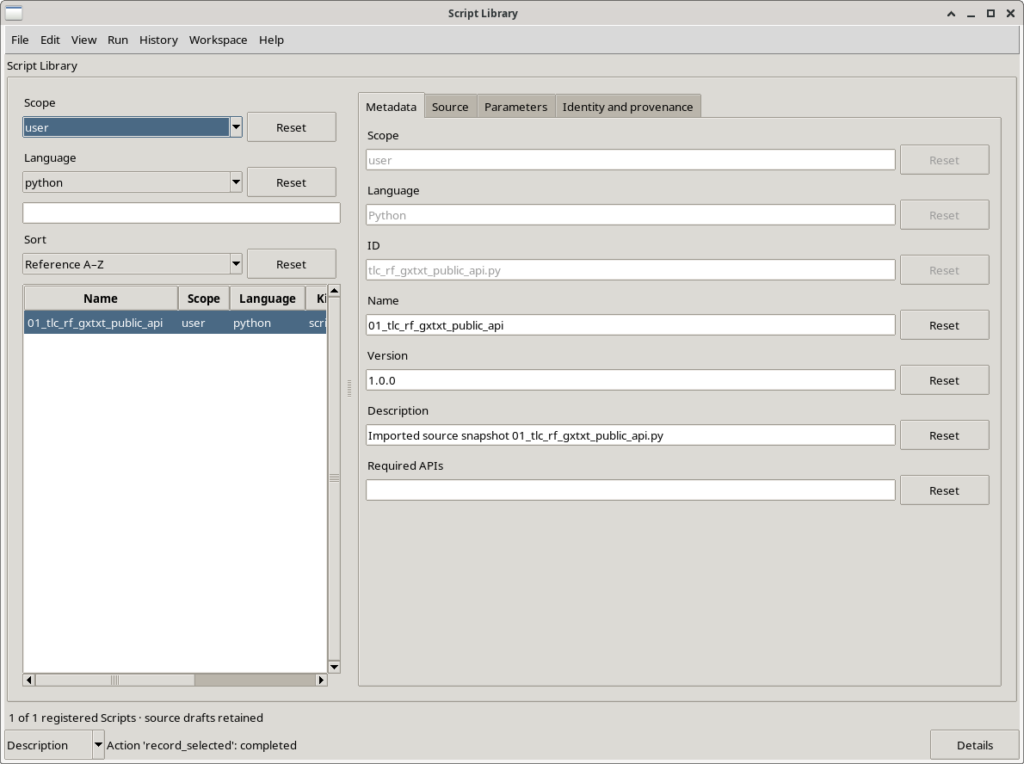
- Import the script into GX-TXT through the Script Library, for example into User Space. This makes it possible to store and reuse it in different Sessions.
- Open the Script Runner for the selected script.
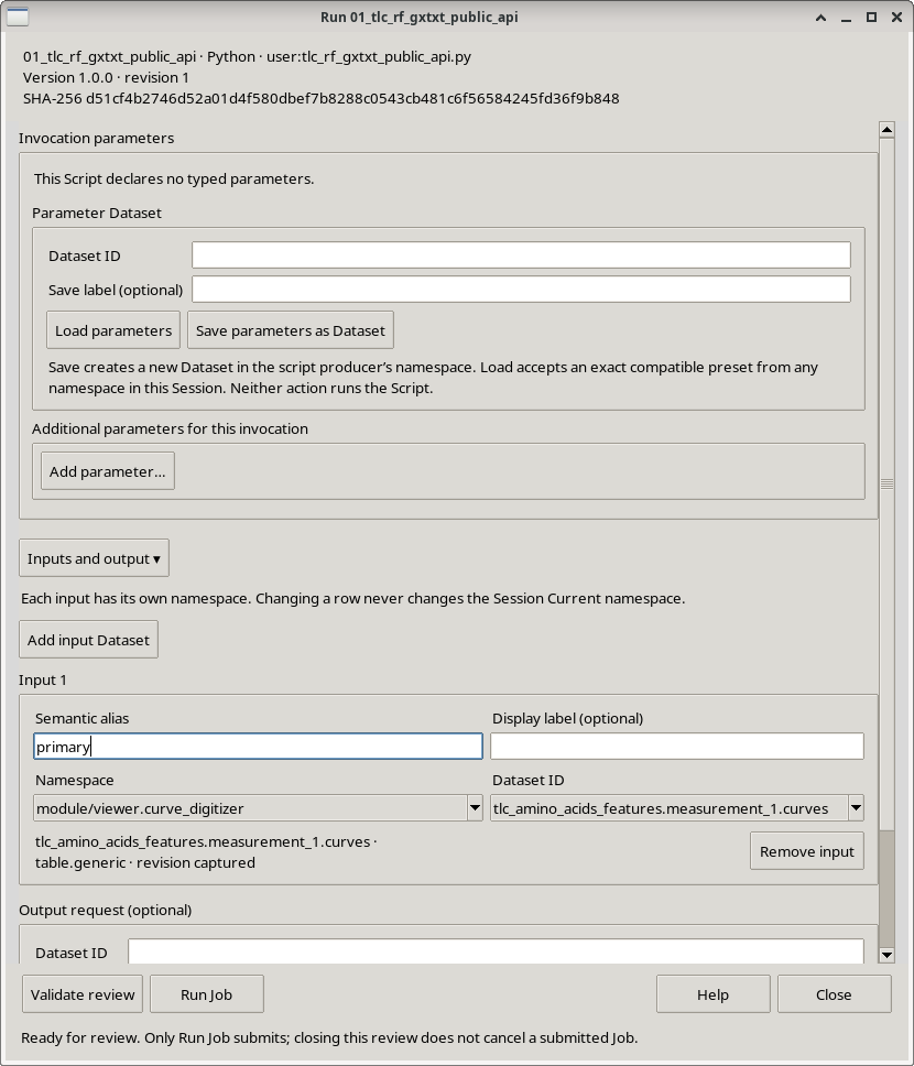
- In Inputs and output, add the Dataset containing the digitized traces and set its Semantic alias to exactly
primary. - Click Validate review, confirm that the correct Dataset is selected, and then choose Run Job.
- Check the Job outcome and open the newly published Dataset containing the retention factors.
primary without hardcoding its identifier in Python.Why the script is reusable
The script obtains the Dataset identifier from the GX-TXT execution context through gxtxt_context(). Technical column identifiers—such as X/Y coordinates, curve identity, and point order—are taken from the metadata published by Curve Digitalizer and checked against the public Variable Schema API. The records are then retrieved through the Canonical Dataset API.
Consequently, the code does not need to be changed every time GX-TXT assigns a different Dataset identifier or different technical column names. The analysis depends on the semantic roles declared by the data producer, rather than the position of columns in a CSV file.
The output Dataset is published through Dataset Publication API v2, using the table.generic contract and CSV format, together with scientific metadata and variable descriptors. This makes the measurements easy to inspect both within GX-TXT and with other scientific software.
How to adapt the script to other TLC plates
Only a few parameters need to be changed, and each has a clear purpose:
BASELINE_LABEL: the name of the application baseline, normallyBASELINE.FRONT_LABEL: the name of the solvent-front line, normallySOLVENT_FRONT.SPOT_LABEL_PATTERN: the naming convention used to recognize individual spot regions, for exampleSPOT_L01_S01_TYROSINE.Ldenotes the lane andSthe spot number within that lane.RESULT_VERSION: the output version suffix (v2,v3, and so on). Changing it allows a new analysis to be published without overwriting an earlier result.- Polygon validation settings, including the maximum acceptable closure gap and the source row limit, can be adjusted for larger or smaller experiments while preserving the consistency checks.
The number of lanes and spots is not hardcoded: a lane can contain multiple spots, as it does in our mixture. The two reference lines and a consistent naming convention recognized by the script are still required. The points describing an outline must belong to one region and follow its boundary in order.
The scientific interpretation must always be checked. A generic script may process its input data correctly, but it cannot guarantee that a marker outline coincides with the true chromatographic stain or that the reference lines were identified without ambiguity.
Experimental results
The execution produced a canonical table with five rows and twelve columns, recording the region name, lane number, spot index, centroid, migration distances, area and perimeter of each annotated region, and its \(R_f\) value.
| Lane and region | \(R_f\) |
|---|---|
| 1 — tyrosine | 0.797371 |
| 2 — glycine | 0.498253 |
| 3 — methionine | 0.698825 |
| 4 — glycine, lower spot | 0.456785 |
| 4 — methionine, upper spot | 0.693192 |
These values come from the actual Dataset published by GX-TXT; the table was not recreated with artificial numbers for this tutorial.
The two methionine readings from lanes 3 and 4 are close (approximately 0.699 and 0.693). The two readings attributed to glycine differ more noticeably (about 0.498 and 0.457). This comparison demonstrates the value of quantitative measurements, but it is not an analytical validation of the mixture’s composition. The results depend on the placement of the marked outlines, centroid calculation, calibration, and interpretation of the solvent front.
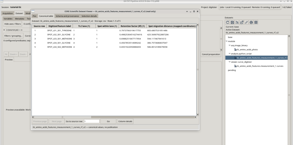
table.generic Dataset stores five Rf measurements together with centroid coordinates and migration distances.Plotting the retention factors
No additional Python code is needed to plot the retention factors. The CORE Scientific Dataset Viewer lets us select the Dataset’s variables explicitly.
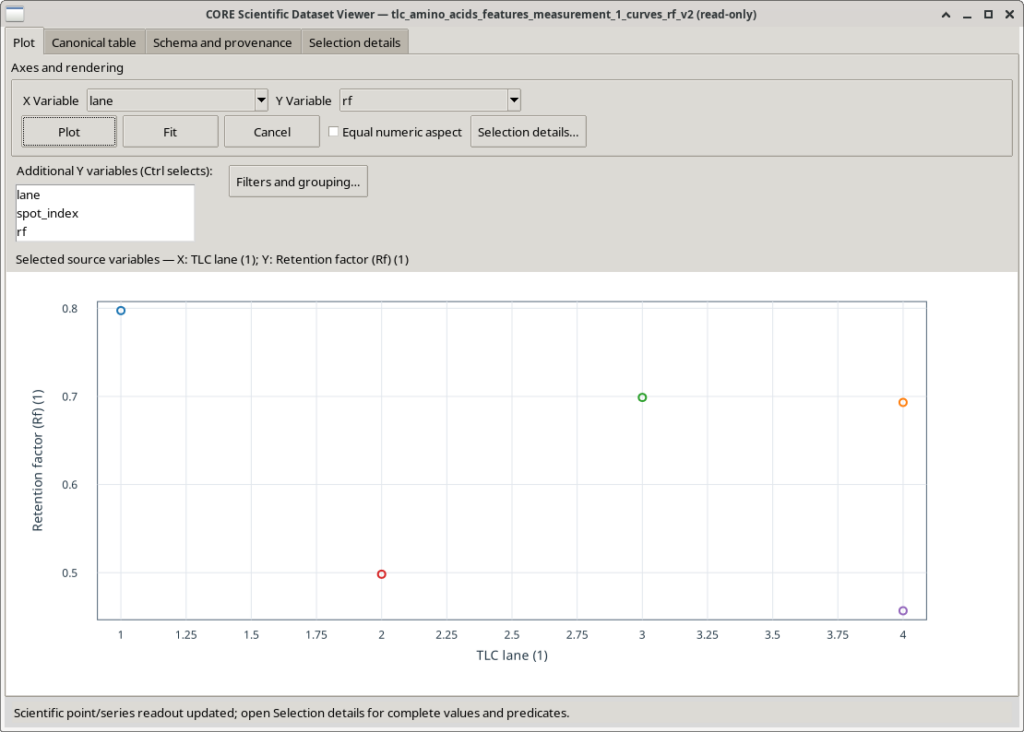
After opening the Dataset, we selected X Variable = lane and Y Variable = rf in the Plot tab. In Filters and grouping…, we separated the observations by feature_name so each spot appears as an independent point rather than joining unrelated observations with a continuous line.
The resulting chart contains five points across four lanes. Two observations appear in lane 4, corresponding to the mixture. This concise visualization makes it easy to compare the relative movement attributed to the reference substances and the mixed sample.
Because this Dataset contains several numerical variables and one text field, the embedded Preview in the main window does not necessarily choose suitable axes automatically. The Dataset Viewer, by contrast, allows the user to specify the variables and inspect both the canonical table and the variable schema.
Results, metadata, and methodological notes
The numerical table is a table.generic Dataset with structured scientific metadata describing the origin of the measurements, the calculation method, coordinate reference, and declared limitations. Longer explanations can be kept in a separate Markdown document.
To make these notes available in GX-TXT, we used a second, optional script, tlc_rf_notes_group_bridge.py. It selects the \(R_f\) results Dataset through the primary input alias, publishes a supporting Markdown document, and creates a Dataset Group containing both resources. The table remains the group’s primary Dataset and is not modified.
#!/usr/bin/env python3
# SPDX-License-Identifier: GPL-3.0-or-later
"""Optional Script Bridge compatibility: TLC result + Markdown Dataset Group.

Select the already published table.generic Rf results as input alias primary.
The existing numeric Dataset is never rewritten. A new supporting Markdown
Dataset is published with the public file publication API, and both Dataset
IDs are linked by the public producer-scoped Dataset Group API. This is not
a substitute for native Dataset Notes and is explicitly labelled as such.
"""

from __future__ import annotations

import hashlib
from pathlib import Path
import re

from gxtxt import gxtxt_api_call, gxtxt_api_require, gxtxt_context

SOURCE_ALIAS = "primary"
VERSION = "v1"


def call(api_id, operation, args):
    return gxtxt_api_call(api_id, operation, args)


def source_from_context(ctx):
    ds = str((ctx.get("inputs", {}).get(SOURCE_ALIAS, {}) or {})
             .get("dataset_id", "")).strip()
    if not re.fullmatch(r"[A-Za-z][A-Za-z0-9_.-]{0,255}", ds):
        raise RuntimeError("Select a canonical TLC results Dataset as primary")
    return ds


def output_ids(ds):
    stem = re.sub(r"[^A-Za-z0-9_.-]", "_", ds)
    if len(stem) > 185:
        stem = stem[:168].rstrip("_.-") + "_" + hashlib.sha256(
            ds.encode("utf-8")).hexdigest()[:12]
    return stem + "_method_notes_" + VERSION, stem + "_with_notes_" + VERSION


def flatten(block, var_id):
    src = block[var_id]["values"]
    if hasattr(src, "reshape"):
        return src.reshape(-1).tolist()
    out = []
    for cell in src:
        if isinstance(cell, (tuple, list)):
            if len(cell) != 1:
                raise ValueError("Expected scalar canonical table variable")
            cell = cell[0]
        out.append(cell)
    return out


def load_table(ds):
    info = call("CANONICAL_DATASET_API_v2", "describe", [ds])
    if info.get("contract") != "table.generic":
        raise RuntimeError("This is not a canonical table.generic Dataset")
    metadata = call("DATASET_METADATA_API_v1", "read", [ds])
    if metadata.get("processing.kind") != "tlc_retention_factor_from_annotated_polygons":
        raise RuntimeError("This Dataset is not a published TLC Rf analysis")
    schema = call("DATASET_VARIABLE_SCHEMA_API_v3", "list", [ds])
    vars_by_id = {str(v["variable_id"]): v for v in schema}
    selected = ("feature_name", "lane", "spot_index", "rf")
    if any(k not in vars_by_id for k in selected):
        raise RuntimeError("Missing TLC source columns: feature_name/lane/spot_index/rf")
    n = int(info.get("row_count", 0))
    if not 1 <= n <= 10000:
        raise RuntimeError("Invalid TLC row count")
    records = []
    for start in range(0, n, 400):
        width = min(400, n-start)
        batch = call("CANONICAL_DATASET_API_v2", "read_range",
                     [ds, list(selected), start, width])
        columns = {k: flatten(batch, k) for k in selected}
        if any(len(v) != width for v in columns.values()):
            raise RuntimeError("Incomplete canonical TLC table")
        for j in range(width):
            records.append({k: columns[k][j] for k in selected})
    return metadata, records


def build_markdown(ds, metadata, records):
    lines = [
        "# TLC — retention factors and methodological notes",
        "",
        "## Origin and interpretation",
        "",
        "Result table: " + ds,
        "",
        "Regions were traced following the hand-drawn marker outlines placed",
        "by a chemist around spots on the source photograph. They are annotated",
        "regions of interest, not objectively segmented color boundaries.",
        "Chemical labels are those supplied by the source, not independently",
        "verified analyte identities.",
        "",
        "## Retention factors",
        "",
        "| Spot label | Lane | Spot | Rf |",
        "| --- | ---: | ---: | ---: |",
    ]
    for r in records:
        label = str(r["feature_name"]).replace("|", "/").replace("\n", " ")
        lines.append("| " + label + " | " + str(int(r["lane"])) + " | " +
                     str(int(r["spot_index"])) + " | " +
                     format(float(r["rf"]), ".6f") + " |")
    lines.extend([
        "",
        "## Method",
        "",
        "Rf is the ratio of the annotated polygon-centroid migration distance",
        "to the solvent-front migration distance. Both were calculated in the",
        "same projectively rectified coordinate system with the original",
        "baseline and solvent-front lines.",
        "",
        "Rf is dimensionless. These mapped coordinates do not establish an",
        "absolute or independently certified physical length scale.",
        "",
        "## Structured provenance",
        "",
    ])
    for k in (
        "processing.input_dataset_id",
        "processing.input_coordinate_unit",
        "processing.method",
        "processing.geometry",
        "processing.rf_method",
        "processing.uncertainty",
    ):
        if k in metadata:
            lines.append("- " + k + ": " + str(metadata[k]))
    lines.extend([
        "",
        "## Limitations",
        "",
        "- The upper marked line is assumed to be the solvent front.",
        "- Spot outline interpretation is operator-dependent.",
        "- Faint stains, notably the first lane, are less reliable.",
        "- Identity and concentration are not proven by photographic Rf alone.",
        "- Lens distortion and plate nonplanarity are not independently corrected.",
        "- Measurement uncertainties and propagated Rf uncertainty are not quantified.",
        "",
        "## Framework version note",
        "",
        "At the time of this tutorial the GX-TXT Script Bridge did not expose",
        "the direct Dataset Notes association API. This note was therefore",
        "published as a separate canonical Markdown Dataset and grouped with",
        "the numerical results. Native Script Bridge integration of Dataset",
        "Notes is planned for the final framework; actual availability",
        "depends on the version installed by the reader.",
        "",
    ])
    return "\n".join(lines)


def main():
    for required in (
        "CANONICAL_DATASET_API_v2@2",
        "DATASET_METADATA_API_v1@1",
        "DATASET_VARIABLE_SCHEMA_API_v3@3",
        "DATASET_FILE_PUBLICATION_API_v1@1",
        "DATASET_GROUP_API_v1@1",
    ):
        gxtxt_api_require(required)
    context = gxtxt_context()
    numeric_id = source_from_context(context)
    metadata, rows = load_table(numeric_id)
    note_id, group_id = output_ids(numeric_id)

    existing = call("DATASET_GROUP_API_v1", "list", [])
    for group in existing:
        if group.get("group_id") == group_id:
            raise RuntimeError("This group already exists; do not re-run")
        if any(m.get("dataset_id") == numeric_id for m in group.get("members", [])):
            raise RuntimeError("Numeric Dataset is already in another group")

    output_dir = Path(context["output_dir"]).resolve()
    output_dir.mkdir(parents=True, exist_ok=True)
    file = output_dir / "tlc_rf_group_notes.md"
    file.write_text(build_markdown(numeric_id, metadata, rows), encoding="utf-8")

    file_result = call("DATASET_FILE_PUBLICATION_API_v1", "publish", [{
        "dataset_id": note_id,
        "contract": "document.text",
        "format": "md",
        "source_file": str(file),
        "storage_kind": "text",
        "media_type": "text/markdown",
        "producer_version": "1.0.0",
        "replace_owned": False,
        "source_dataset_ids": [numeric_id],
        "source": "GX-TXT TLC tutorial Python Script Bridge",
        "provenance": "Interpretation of chemist-annotated TLC Rf results",
        "structured_metadata": {
            "documentation.kind": "tlc_method_notes",
            "documentation.for_dataset_id": numeric_id,
            "documentation.association": "dataset_group_compatibility",
            "documentation.direct_dataset_notes_script_api": "not_available_at_tutorial_time",
        },
    }])
    print("TLC_NOTES_DATASET_PUBLISHED", file_result, flush=True)

    definition = {
        "group_id": group_id,
        "display_name": "TLC Rf results and methodological notes",
        "group_contract": "scientific.tlc_rf_results",
        "primary_dataset_id": numeric_id,
        "members": [
            {"dataset_id": numeric_id, "role": "primary.result_table",
             "required": True, "contract": "table.generic"},
            {"dataset_id": note_id, "role": "supporting.method_notes",
             "required": False, "contract": "document.text"},
        ],
    }
    # Review pins actual Session, ownership, Namespace and opaque revisions.
    review = call("DATASET_GROUP_API_v1", "review", [[numeric_id, note_id]])
    receipt = call("DATASET_GROUP_API_v1", "create", [definition, review])
    print("TLC_GROUP_CREATED", receipt, flush=True)


if __name__ == "__main__":
    main()
# TLC retention factor — scientific notes

## Provenance

Source Dataset: tlc_amino_acids_features.measurement_1.curves

Result Dataset: tlc_amino_acids_features_measurement_1_curves_rf_v2

Original Curve Digitalizer rows: 1866

Coordinate unit in source: px

The spot regions were **drawn in marker by a chemist** on the original photograph. We digitized those annotations, not automatically segmented chemical stain boundaries. Chemical names are source labels, not independently verified identities.

## Method

Each annotated contour was treated as a polygon. Its shoelace centroid was projected onto the migration direction, defined as the normal to BASELINE. The solvent front was evaluated at the same baseline-tangent coordinate. Rf equals spot migration distance divided by solvent-front migration distance.

Values are dimensionless; source coordinate units describe a projectively mapped plate, **not a certified physical mm scale**.

## Measured spots

| Source curve name | Lane | Spot | Rf |
|---|---:|---:|---:|
| SPOT_L01_S01_TYROSINE | 1 | 1 | 0.797371 |
| SPOT_L02_S01_GLYCINE | 2 | 1 | 0.498253 |
| SPOT_L03_S01_METHIONINE | 3 | 1 | 0.698825 |
| SPOT_L04_S01_GLYCINE | 4 | 1 | 0.456785 |
| SPOT_L04_S02_METHIONINE | 4 | 2 | 0.693192 |

## Producer semantic role mappings

Resolved from the source's Curve Digitalizer metadata and the public Variable Schema API, not from hardcoded CSV column headers.

- curve_key: curve_id
- curve_name: curve_label
- point_order: point_index
- x: x
- y: y

## Limitations

- The upper reference line is presumed to be the solvent front; its identity requires experimental confirmation.
- A manually drawn perimeter may not coincide exactly with the stain.
- The faint tyrosine region is especially sensitive to operator annotation.
- Rf alone cannot establish chemical identity or concentration.
- Lens distortion and nonplanarity are not corrected by a projective mapping.
- Source-coordinate uncertainties and propagated Rf uncertainties have not been quantified.

This note can be associated via the GX-TXT Dataset Notes editor. It is not a second scientific Dataset.
In the GX-TXT version used for this experiment, Python scripts could not yet attach Markdown notes directly to a Dataset. We therefore used a Dataset Group to keep the numerical results and documentation together. Direct note integration is planned for the final framework release; readers should check which workflow is supported by their installed version.
Readers who prefer a simpler workflow can download the Markdown document from this article and read it separately, without using the second script: calculating \(R_f\) does not depend on the notes.
What we achieved and what remains to be verified
This experiment demonstrated an end-to-end workflow: a real photograph, perspective calibration of the TLC plate, digitization of seven curves, publication of their coordinates, Python-based analysis, publication of a results table, and visualization using GX-TXT’s scientific plotting tools.
The most important outcome is not just a final \(R_f\) value, but the traceability of the analysis. The table is derived from annotated regions, retains its relationship to the original curves, and can be reproduced by anyone with the image, GX-TXT, and the scripts. Keeping numerical data separate from scientific commentary also makes the results easier to reuse in subsequent analyses.
The limitations of this example should remain explicit: the spot boundaries were marked by the chemist, the tyrosine stain is faint, the solvent front is interpreted from the source, and measurement uncertainties were not quantified. Agreement between two \(R_f\) values suggests geometric consistency, but does not by itself establish the identity of a compound.
Possible extensions include comparing the annotated centroids with positions extracted through color segmentation, repeating the digitization independently, or introducing uncertainty models for the baseline, solvent front, and spot outlines. Each would extend the same basic principle: start with an observable measurement and document precisely what the evidence can—and cannot—support.
Photograph source and license: Amino acids TLC with English translation, Dvnyn, adapted from TheFatDrummer, Wikimedia Commons, CC BY-SA 4.0. This article uses a crop of the photographic portion of the original composite.