GX-TXT Curve Digitalizer: From a Titration Curve to the Equivalence Point with Python

14 November 2026 di Giux GX-TXT 19 min di lettura

In this tutorial, we demonstrate a complete workflow with GX-TXT Curve Digitalizer applied to an acid–base titration curve. Starting from a published graph, we digitize the experimental data points, publish a scientific Dataset, and use a Python script based on the public GX-TXT APIs to reconstruct a smoothed numerical curve, calculate its d(pH)/dV derivative, and estimate the equivalence point.

The aim is not simply to extract coordinates from an image, but to show how Curve Digitalizer can become the first stage of a reproducible scientific analysis: from the original figure to a Dataset, from the Dataset to numerical processing, and finally to native charts in the Plots window.

Source graph and experimental setup

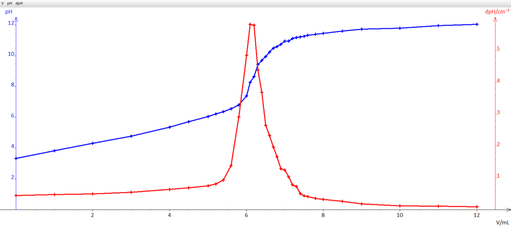
The source for this experiment is a titration curve showing pH as a function of the volume of NaOH added. After importing the image into Curve Digitalizer, we performed the standard axis calibration and digitized the points by selecting the centers of the markers shown in the original graph.

Because the source figure uses graphical symbols rather than explicitly defined error bars, we did not interpret the width of each cross as a documented uncertainty. The extracted points therefore represent a carefully digitized version of the published curve. They are suitable for subsequent analysis but are not equivalent to primary measurements taken directly in a laboratory.

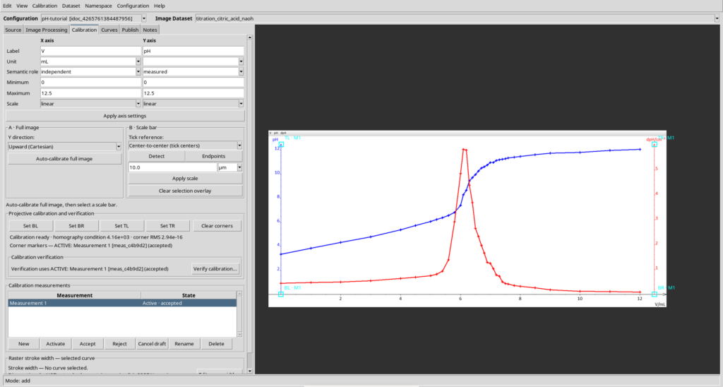
Citric acid titration graph showing the blue pH curve and red pH derivative plotted against the volume of NaOH titrant. — Original citric acid titration graph used as the digitization source. Anhmaidq, Wikimedia Commons, CC BY-SA 4.0.

Calibrating volume and pH correctly

After importing the graph as an Image Dataset, we open the Calibration tab and set X to the NaOH volume in mL and Y to pH. Both plotted axes are linear: although pH is defined logarithmically in chemistry, that does not mean the pH values appear on a logarithmic plot axis. The four-reference-point calibration was accepted before the curve was digitized.

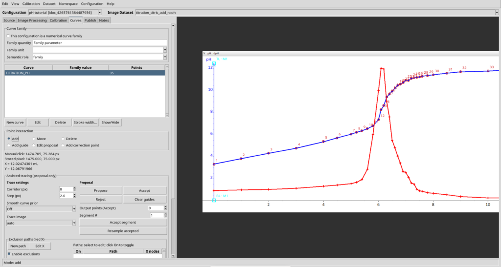
GX-TXT Curve Digitalizer Calibration interface showing a titration graph, an X axis in mL, a pH Y axis, and four calibration points. — Four-point calibration of the titration graph in GX-TXT, with linear volume and pH axes.

Digitizing the 35 points of the blue curve

In the Curves tab, we created a single independent curve named TITRATION_PH. We captured 35 points by following the centers of the blue crosses, with denser sampling around the steep pH rise. The points are ordered by increasing volume. The red derivative curve already present in the source image was not digitized: it is retained only as a reference for comparison with our computed result.

GX-TXT Curves tab showing 35 digitized points along the blue titration curve, with denser sampling near the steep pH transition. — Acquisition of the 35 TITRATION_PH points by selecting the centers of the crosses in the original graph.

From Curve Digitalizer to a scientific Dataset

After digitization, we publish the curve as a scientific Dataset. The data are no longer merely a list of exported coordinates: they become a structured object within the framework, with an identity, metadata, and interoperability with other GX-TXT tools.

In this example, the source Dataset contains the volume–pH points extracted from the figure. A Python script then processes this Dataset using only public APIs available through script_bridge: it reads the data, constructs a smoothed numerical representation, calculates the derivative, and publishes a second Dataset containing the analysis results.

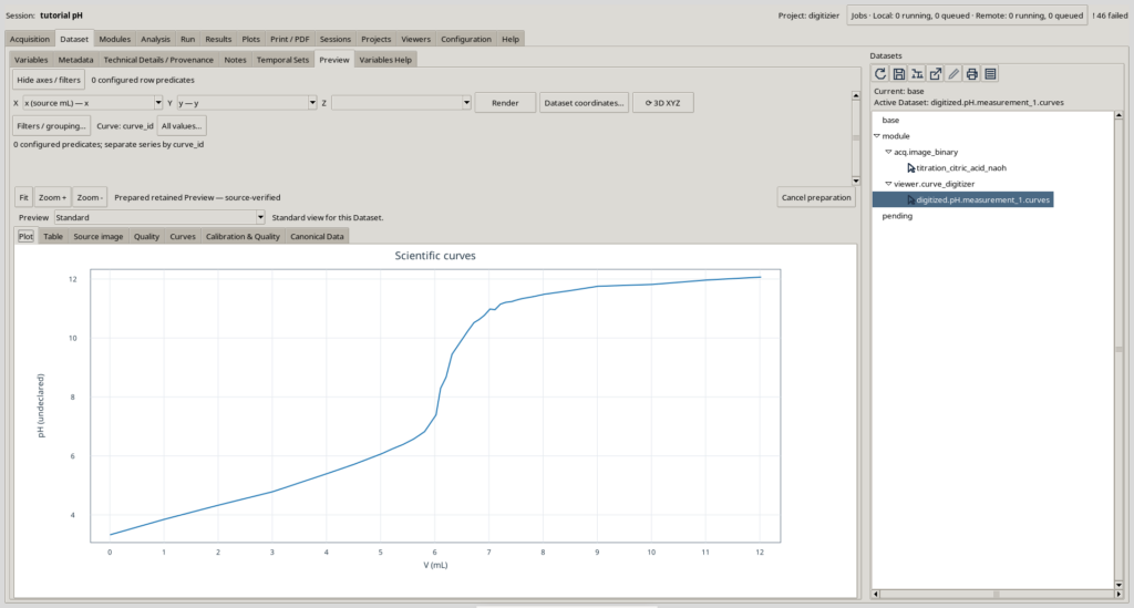
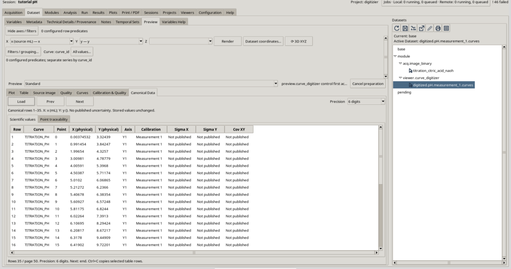
pH versus NaOH volume curve shown in GX-TXT Dataset Preview, reconstructed from 35 digitized data points. — The titration curve published as a GX-TXT scientific Dataset, plotted against volume and pH axes.

The canonical table displays the 35 volume–pH pairs actually digitized. The uncertainty columns Sigma X, Sigma Y, and Cov XY are marked Not published. We did not infer measurement uncertainties from the graphical dimensions of the crosses.

GX-TXT table containing 35 digitized volume–pH coordinates, with Sigma X, Sigma Y and Cov XY marked Not published. — The 35 volume–pH pairs in the canonical Dataset. Undocumented uncertainties were not published.

Numerical analysis with Python: smoothed curve, derivative, and equivalence point

The analysis script takes the digitized Dataset as a generic input, without depending on fixed local file paths. Through the framework’s public APIs, it reads the variable identities and metadata, interpolates and smooths the curve, and creates a denser numerical profile from which the d(pH)/dV derivative can be estimated.

An apparent equivalence point is then estimated from the maximum of the numerical derivative. In mathematical terms, we seek the volume V at which this derivative reaches its maximum:

\[ V_{\mathrm{eq,app}}=\operatorname*{arg\,max}_{V}\left(\frac{d(\mathrm{pH})}{dV}\right) \]

This procedure is not a substitute for a complete metrological analysis, but it is useful for turning a published curve into numerical data that can be examined, compared, and reproduced.

No screenshot of the script is needed for this step. The complete code actually executed is available in the expandable section below.

The script processed the 35 points published in GX-TXT and created a second table.generic Dataset in CSV format, with the variables volume_ml, ph_interpolated, ph_smoothed, and dph_dv. Its 2,001 output rows contain interpolated or computed coordinates, not new experimental observations.

Result	Measured or calculated value
Points digitized from the graph	35
Interpolated numerical positions	2,001 (not new measurements)
Derivative maximum with 0.15 mL smoothing	6.134 mL
Range of maximum positions with 0.12–0.18 mL smoothing	6.122–6.146 mL (numerical sensitivity only)
Apparent equivalence volume to report	approximately 6.1 mL

The calculated maximum occurs at 6.134 mL. The variation in its location with different smoothing widths is not a measurement of experimental uncertainty. Given the resolution of the source figure, the scientifically cautious conclusion is an apparent equivalence volume of approximately 6.1 mL. Citric acid is polyprotic: the maximum alone is not sufficient to identify a particular stoichiometric equivalence stage.

Show the complete Python script for numerical analysis

#!/usr/bin/env python3
# SPDX-License-Identifier: GPL-3.0-or-later
"""Estimate an apparent acid-base equivalence volume from digitized pH(V).

Use a single independently digitized curve called TITRATION_PH with X in mL
and Y as linear numeric pH, published as a Curve Digitalizer Dataset.

Script Runner input alias: primary.
Outputs: one canonical table.generic CSV, no extra document Dataset.
The apparent derivative maximum does not establish an exact stoichiometric
equivalence point for a polyprotic acid, nor a statistical uncertainty.
"""
from __future__ import annotations

from collections import defaultdict
from pathlib import Path
from hashlib import sha256
import json
import re

import numpy as np
from scipy.interpolate import PchipInterpolator
from scipy.ndimage import gaussian_filter1d
from gxtxt import gxtxt_api_call, gxtxt_api_require, gxtxt_context

SOURCE_ALIAS = "primary"
CURVE_LABEL = "TITRATION_PH"
OUTPUT_VERSION = "v1"
MIN_SOURCE_POINTS = 25  # Source GUI actually contains 35 independently digitized points.
MAX_SOURCE_ROWS = 100000
GRID_POINTS = 2001
SIGMA_ML = 0.15  # Reduces PCHIP derivative ripples from sparse marks.
SIGMA_CHECKS_ML = (0.12, 0.15, 0.18)

REQUIRED_APIS = [
    "CANONICAL_DATASET_API_v2@2",
    "DATASET_METADATA_API_v1@1",
    "DATASET_VARIABLE_SCHEMA_API_v3@3",
    "DATASET_PUBLICATION_API_v2@2",
]

OUTPUT_VARIABLES = (
    ("volume_ml", "Titrant volume", "mL"),
    ("ph_interpolated", "pH interpolated from digitized points", "1"),
    ("ph_smoothed", "Numerically smoothed pH", "1"),
    ("dph_dv", "Numerical derivative of pH with respect to volume", "1/mL"),
)


def api(owner, operation, args):
    return gxtxt_api_call(owner, operation, args)


def selected_dataset(ctx):
    src = str((ctx.get("inputs", {}).get(SOURCE_ALIAS, {}) or {})
              .get("dataset_id", "")).strip()
    if not src:
        raise RuntimeError("Select a Curve Digitalizer Dataset as input primary")
    return src


def output_id(source):
    stem = re.sub(r"[^a-z0-9_]+", "_", source.lower()).strip("_")
    if len(stem) > 65:
        stem = stem[:52].rstrip("_") + "_" + sha256(
            source.encode("utf-8")).hexdigest()[:10]
    if not stem or not re.fullmatch(r"v[1-9][0-9]*", OUTPUT_VERSION):
        raise RuntimeError("Invalid source identity or output version")
    return stem + "_titration_eq_" + OUTPUT_VERSION


def unpack_column(block, variable_id):
    v = block[variable_id]["values"]
    if hasattr(v, "reshape"):
        return v.reshape(-1).tolist()
    out = []
    for cell in v:
        if isinstance(cell, (list, tuple)):
            if len(cell) != 1:
                raise RuntimeError("Scalar column expected")
            cell = cell[0]
        out.append(cell)
    return out


def digitized_curve(source):
    """Map producer semantic roles through public Dataset metadata and schema."""
    md = api("DATASET_METADATA_API_v1", "read", [source])
    if md.get("curve_digitizer.plugin_id") != "viewer.curve_digitizer":
        raise RuntimeError("Expected Curve Digitalizer source provenance")
    if md.get("curve_digitizer.curve_mode") != "independent":
        raise RuntimeError("Use independent curve mode")
    if md.get("curve_digitizer.curve_grouping") != "curve_key":
        raise RuntimeError("Use the selected single-calibration Dataset")

    desc = api("CANONICAL_DATASET_API_v2", "describe", [source])
    if desc.get("contract") != "table.generic":
        raise RuntimeError("Expected table.generic Dataset")
    row_count = int(desc.get("row_count", 0))
    if not MIN_SOURCE_POINTS <= row_count <= MAX_SOURCE_ROWS:
        raise RuntimeError("Unexpected number of digitized source points")

    schema = api("DATASET_VARIABLE_SCHEMA_API_v3", "list", [source])
    by_id = {str(c["variable_id"]): c for c in schema}
    roles = ("x", "y", "curve_key", "curve_name", "point_order")
    dimension = str(md.get("curve_digitizer.curve_row_dimension", ""))
    if not dimension:
        raise RuntimeError("Curve row dimension metadata missing")
    columns = {}
    for role in roles:
        var = str(md.get("curve_digitizer.curve_column." + role, "")).strip()
        if not var or var not in by_id:
            raise RuntimeError("No public source variable for role " + role)
        entry = by_id[var]
        dims = entry.get("dimension_ids", "")
        dims = list(dims) if isinstance(dims, (list, tuple)) else str(
            dims).replace(";", " ").split()
        if str(entry.get("rank")) != "1" or dims != [dimension]:
            raise RuntimeError("Variable rank/dimension mismatch: " + role)
        columns[role] = var
    if len(set(columns.values())) != len(columns):
        raise RuntimeError("Overlapping semantic variable mappings")

    x_unit = str(by_id[columns["x"]].get("unit", ""))
    y_unit = str(by_id[columns["y"]].get("unit", ""))
    if x_unit != "mL" or y_unit not in ("1", "pH", ""):
        raise RuntimeError("Expected linear volume in mL and numeric pH")
    # A blank source Y unit means dimensionless pH in the actual GUI figure.
    # Validate the explicit calibrated axis labels rather than guessing.
    raw_calibrations = md.get("curve_digitizer.calibration_measurements", "")
    if not raw_calibrations:
        raise RuntimeError("Missing source calibration axis descriptions")
    calibrations = (
        json.loads(raw_calibrations)
        if isinstance(raw_calibrations, str) else raw_calibrations
    )
    accepted = [
        item for item in calibrations
        if item.get("state") == "accepted" and item.get("active")
    ]
    if len(accepted) != 1:
        raise RuntimeError("Expected one active accepted calibration")
    axes = accepted[0].get("axes", {})
    ax_x, ax_y = axes.get("x", {}), axes.get("y", {})
    if (ax_x.get("scale") != "linear" or
        ax_y.get("scale") != "linear" or
        ax_x.get("unit") != "mL" or
        str(ax_y.get("name", "")).lower() != "ph"):
        raise RuntimeError("Expected a linear volume and linear pH calibration")

    groups = defaultdict(list)
    labels = {}
    requested = list(dict.fromkeys(columns.values()))
    for start in range(0, row_count, 1000):
        count = min(1000, row_count - start)
        block = api("CANONICAL_DATASET_API_v2", "read_range",
                    [source, requested, start, count])
        data = {k: unpack_column(block, c) for k, c in columns.items()}
        if any(len(v) != count for v in data.values()):
            raise RuntimeError("Incomplete canonical read_range response")
        for i in range(count):
            key = str(data["curve_key"][i]).strip()
            label = str(data["curve_name"][i]).strip().upper()
            order = int(data["point_order"][i])
            x, y = float(data["x"][i]), float(data["y"][i])
            if not key or not label or not (np.isfinite(x) and np.isfinite(y)):
                raise RuntimeError("Invalid digitized point")
            if key in labels and label != labels[key]:
                raise RuntimeError("Inconsistent name assigned to source curve")
            labels[key] = label
            groups[key].append((order, x, y))
    matches = [k for k, label in labels.items() if label == CURVE_LABEL]
    if len(matches) != 1:
        raise RuntimeError("Expected exactly one curve named " + CURVE_LABEL)
    ordered = sorted(groups[matches[0]])
    if [row[0] for row in ordered] != list(range(len(ordered))):
        raise RuntimeError("Point sequence is not contiguous and zero-based")
    return (
        np.array([row[1] for row in ordered], dtype=np.float64),
        np.array([row[2] for row in ordered], dtype=np.float64),
        columns, row_count,
    )


def derivative_analysis(volume, ph):
    """PCHIP regularization, Gaussian smoothing and d(pH)/dV peak search."""
    x = np.asarray(volume, dtype=np.float64)
    y = np.asarray(ph, dtype=np.float64)
    if x.ndim != 1 or x.size != y.size or x.size < MIN_SOURCE_POINTS:
        raise ValueError("At least 40 pH(V) points are required")
    if not np.all(np.isfinite(x)) or not np.all(np.isfinite(y)):
        raise ValueError("Nonfinite source point")
    if not np.all(np.diff(x) > 0):
        raise ValueError(
            "Volume must be strictly increasing; correct any duplicated or "
            "backward X points near the steep section in Curve Digitalizer")
    if np.min(y) < 0 or np.max(y) > 14.5:
        raise ValueError("Unexpected pH range")
    span = float(x[-1] - x[0])
    if span < 2.5:
        raise ValueError("Digitized volume interval is too short")
    if np.sum(np.diff(y) < -0.25) > max(4, int(0.04 * len(y))):
        raise ValueError("Expected predominantly rising pH curve")

    grid = np.linspace(float(x[0]), float(x[-1]), GRID_POINTS)
    step = float(grid[1] - grid[0])
    ph_interpolated = PchipInterpolator(x, y)(grid)
    inside = (grid >= grid[0] + 0.05 * span) & (
        grid <= grid[-1] - 0.05 * span)
    candidates = np.where(inside)[0]

    positions = {}
    curves = {}
    for sigma in sorted(set((*SIGMA_CHECKS_ML, SIGMA_ML))):
        ph_smooth = gaussian_filter1d(
            ph_interpolated, sigma / step, mode="nearest")
        derivative = np.gradient(ph_smooth, grid)
        peak = int(candidates[np.argmax(derivative[candidates])])
        if derivative[peak] <= 0:
            raise ValueError("No positive derivative maximum was found")
        positions[sigma] = float(grid[peak])
        curves[sigma] = (ph_smooth, derivative)

    ph_smoothed, dph_dv = curves[SIGMA_ML]
    eq = positions[SIGMA_ML]
    eq_index = int(np.argmin(np.abs(grid - eq)))
    return {
        "volume_ml": grid,
        "ph_interpolated": ph_interpolated,
        "ph_smoothed": ph_smoothed,
        "dph_dv": dph_dv,
        "eq_ml": eq,
        "eq_ph": float(ph_smoothed[eq_index]),
        "peak_dph_dv": float(dph_dv[eq_index]),
        "sensitivity_lo_ml": min(positions.values()),
        "sensitivity_hi_ml": max(positions.values()),
        "source_points": int(x.size),
    }


def publish(source, destination, result, columns):
    metadata = {
        "processing.kind": "titration_ph_derivative_maximum",
        "processing.source_dataset_id": source,
        "processing.source_curve": CURVE_LABEL,
        "processing.source_roles": json.dumps(columns, sort_keys=True),
        "processing.source_points": str(result["source_points"]),
        "processing.axis_x": "linear_volume_mL",
        "processing.axis_y": "linear_numeric_pH",
        "processing.derivative_method": "pchip_gaussian_smoothed_gradient",
        "processing.grid_points": str(GRID_POINTS),
        "processing.sigma_ml": str(SIGMA_ML),
        "processing.sensitivity_sigmas_ml": json.dumps(SIGMA_CHECKS_ML),
        "processing.apparent_eq_volume_ml": format(result["eq_ml"], ".8f"),
        "processing.apparent_eq_ph": format(result["eq_ph"], ".8f"),
        "processing.apparent_max_dph_dv": format(result["peak_dph_dv"], ".8f"),
        "processing.sensitivity_lo_ml": format(
            result["sensitivity_lo_ml"], ".8f"),
        "processing.sensitivity_hi_ml": format(
            result["sensitivity_hi_ml"], ".8f"),
        "processing.sensitivity_kind":
            "smoothing_parameter_not_statistical_uncertainty",
        "processing.chemical_interpretation":
            "apparent_derivative_peak_not_stoichiometric_assignment",
        "processing.uncertainty": "not_quantified",
    }
    request = {
        "dataset_id": destination,
        "contract": "table.generic",
        "storage": "csv",
        "replace_owned": True,  # Explicit same-producer revision; no extra Dataset.
        "producer_version": "1.0.0",
        "source_dataset_ids": [source],
        "source": "GX-TXT Python Script Workspace public Script Bridge",
        "provenance": "Derivative from the original digitized titration pH curve",
        "structured_metadata": metadata,
    }
    writer = api("DATASET_PUBLICATION_API_v2", "begin", [request])
    try:
        api("DATASET_PUBLICATION_API_v2", "declare_dimension",
            [writer, "row", 0, {"extendible": True}])
        table = {}
        for name, label, unit in OUTPUT_VARIABLES:
            descriptor = {
                "dtype": "float64", "rank": 1,
                "dimension_ids": "row",
                "coordinate_role":
                    "coordinate" if name == "volume_ml" else "data",
                "name": name, "display_label": label,
                "unit": unit, "semantic_role":
                    "independent" if name == "volume_ml" else "derived",
            }
            api("DATASET_PUBLICATION_API_v2", "declare_variable",
                [writer, name, descriptor])
            table[name] = [float(v) for v in result[name]]
        api("DATASET_PUBLICATION_API_v2", "append", [writer, "row", table])
        receipt = api("DATASET_PUBLICATION_API_v2", "finalize", [writer])
        writer = None
        return receipt
    except Exception:
        if writer is not None:
            api("DATASET_PUBLICATION_API_v2", "abort", [writer])
        raise


def main():
    gxtxt_api_require(REQUIRED_APIS)
    ctx = gxtxt_context()
    source = selected_dataset(ctx)
    x, y, roles, count = digitized_curve(source)
    result = derivative_analysis(x, y)
    print("TITRATION_SOURCE", source, "source_rows", count, flush=True)
    print("APPARENT_EQ_VOLUME_ML", format(result["eq_ml"], ".5f"), flush=True)
    print("SMOOTHING_SENSITIVITY_ML",
          format(result["sensitivity_lo_ml"], ".5f"),
          format(result["sensitivity_hi_ml"], ".5f"), flush=True)
    receipt = publish(source, output_id(source), result, roles)
    print("TITRATION_DATASET_PUBLISHED", receipt, flush=True)
    folder = Path(ctx["output_dir"]).resolve()
    folder.mkdir(parents=True, exist_ok=True)
    (folder / "titration_summary.md").write_text(
        "# Titration result\n\n"
        + "Apparent derivative-peak volume: "
        + format(result["eq_ml"], ".5f") + " mL.\n\n"
        + "Smoothing sensitivity range: "
        + format(result["sensitivity_lo_ml"], ".5f") + " to "
        + format(result["sensitivity_hi_ml"], ".5f") + " mL.\n\n"
        + "These are not statistical uncertainty bounds. For a polyprotic "
        + "acid, the isolated peak does not identify a particular "
        + "stoichiometric equivalence or analyte concentration.\n",
        encoding="utf-8",
    )


if __name__ == "__main__":
    main()

Two charts in the Plots window: original and smoothed data

To display the results clearly, we used a second Python script, also based on the framework’s public APIs. It creates two persistent charts in the Plots window through Plot Dataset API v4. This avoids relying on Dataset Preview and instead uses GX-TXT’s native plotting system.

The first chart shows the 35 original digitized points on the left Y axis and the numerical derivative on the right Y axis. The second chart shows the smoothed pH curve, again compared with the same numerical derivative. Together, the charts make it easy to compare the values extracted from the original figure with the numerically processed result.

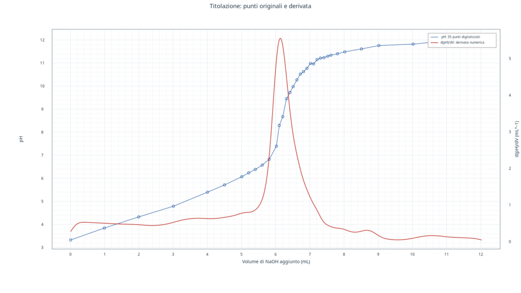
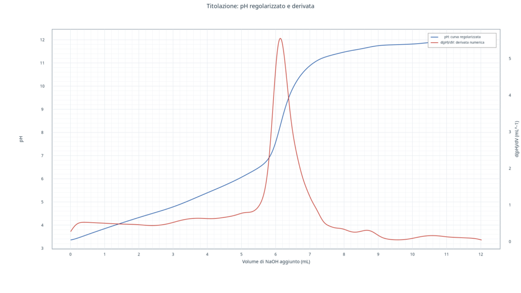
GX-TXT dual-Y-axis chart showing 35 original pH points in blue and the numerical derivative in red against NaOH volume. — First native Plot Dataset v4 chart: the 35 digitized points on the left Y axis and the numerical derivative on the right.

GX-TXT dual-Y-axis chart displaying the smoothed pH curve in blue and the numerical derivative in red, peaking near 6.1 mL. — Second native GX-TXT chart: smoothed pH curve and d(pH)/dV derivative, with a maximum near 6.1 mL.

This workflow also illustrates an important GX-TXT capability: a Python script can do more than process data. It can create persistent charts that can be reopened in the GUI, updated on subsequent runs, and managed by the framework’s plotting system.

Show the complete Python script for the two 2D charts

#!/usr/bin/env python3
# SPDX-License-Identifier: GPL-3.0-or-later
"""Create two persistent Plot Dataset v4 dual-Y charts from existing GX-TXT data.

Script Runner input alias 'primary': the Python-produced titration result
Dataset, with volume_ml, ph_smoothed, ph_interpolated and dph_dv variables.
The source 35-point Curve Digitalizer Dataset is resolved from the published
processing.source_dataset_id metadata; no Session path or Dataset ID is fixed.

Graph 1: original digitized pH points (left Y) and derivative (right Y).
Graph 2: smoothed pH (left Y) and derivative (right Y).
No Dataset is created or modified. Re-running updates these same two Variants.
"""

from gxtxt import gxtxt_api_call, gxtxt_api_require, gxtxt_context

PLOT_API = "PLOT_DATASET_API_v4"
RESULT_ALIAS = "primary"
GRAPH = "plot.dataset.xy"


def api(name, operation, *args):
    return gxtxt_api_call(name, operation, list(args))


def variable_ids(dataset_id, required):
    variables = api("DATASET_VARIABLE_SCHEMA_API_v3", "list", dataset_id)
    by_id = {str(item["variable_id"]): item for item in variables}
    missing = [name for name in required if name not in by_id]
    if missing:
        raise RuntimeError(
            "Dataset " + dataset_id + " lacks variables: " + ", ".join(missing))
    return by_id


def series(id_, dataset, xvar, yvar, side, label, kind, color):
    return {
        "id": id_,
        "dataset_id": dataset,
        "x_variable_id": xvar,
        "y_variable_id": yvar,
        "axis": side,
        "kind": kind,
        "label": label,
        "style": {
            "color": color,
            "line_width": 1.9 if kind != "line_marker" else 1.3,
            "marker": "circle" if kind == "line_marker" else "none",
            "marker_size": 3.8 if kind == "line_marker" else 4,
        },
    }


def plot_spec(title, pH_series, derivative_series):
    spec = api(PLOT_API, "new_spec", GRAPH, title)
    panels = spec["panels"]
    if len(panels) != 1:
        raise RuntimeError("Expected a single default PlotSpec panel")
    panel = panels[0]
    panel["title"] = ""
    panel["axes"] = {
        "x": {"label": "Volume di NaOH aggiunto (mL)", "scale": "linear"},
        "y_left": {"label": "pH", "scale": "linear"},
        "y_right": {"label": "d(pH)/dV (mL^-1)", "scale": "linear"},
    }
    panel["series"] = [pH_series, derivative_series]
    panel["annotations"] = []
    spec["panels"] = [panel]
    return spec


def make_plot(key, spec):
    valid = api(PLOT_API, "validate_spec", spec)
    if not valid:
        raise RuntimeError("PlotSpec validation failed: " + key)
    ref = api(PLOT_API, "upsert_plot", key, spec)
    print("PLOT_VARIANT_REGISTERED", key, ref, flush=True)
    rendered = api(PLOT_API, "render", ref)
    print("PLOT_RENDER_RESULT", key, rendered, flush=True)
    available = api(PLOT_API, "artifacts", ref)
    print("PLOT_ARTIFACTS", key, available, flush=True)
    return ref


def main():
    gxtxt_api_require([
        "PLOT_DATASET_API_v4@4",
        "DATASET_METADATA_API_v1@1",
        "DATASET_VARIABLE_SCHEMA_API_v3@3",
        "CANONICAL_DATASET_API_v2@2",
    ])
    context = gxtxt_context()
    analysis_id = str(
        (context.get("inputs", {}).get(RESULT_ALIAS, {}) or {})
        .get("dataset_id", "")).strip()
    if not analysis_id:
        raise RuntimeError("Bind the TITRATION ANALYSIS Dataset as 'primary'")

    info = api("CANONICAL_DATASET_API_v2", "describe", analysis_id)
    metadata = api("DATASET_METADATA_API_v1", "read", analysis_id)
    if info.get("contract") != "table.generic" or \
            metadata.get("processing.kind") != "titration_ph_derivative_maximum":
        raise RuntimeError("Select the numerical titration derivative Dataset")

    source_id = str(metadata.get("processing.source_dataset_id", "")).strip()
    if not source_id:
        raise RuntimeError("Missing original Curve Digitalizer Dataset lineage")
    source_metadata = api("DATASET_METADATA_API_v1", "read", source_id)
    if source_metadata.get("curve_digitizer.plugin_id") != "viewer.curve_digitizer":
        raise RuntimeError("Declared original is not a Curve Digitalizer Dataset")
    x_source = str(source_metadata.get("curve_digitizer.curve_column.x", ""))
    y_source = str(source_metadata.get("curve_digitizer.curve_column.y", ""))
    if not x_source or not y_source:
        raise RuntimeError("Source lacks semantic X/Y mapping")

    result_vars = variable_ids(
        analysis_id, ("volume_ml", "ph_smoothed", "dph_dv", "ph_interpolated"))
    source_vars = variable_ids(source_id, (x_source, y_source))
    if str(result_vars["volume_ml"].get("unit")) != "mL" or \
            str(source_vars[x_source].get("unit")) != "mL":
        raise RuntimeError("Both volume coordinate axes must be in mL")

    original = series(
        "original_ph_marks", source_id, x_source, y_source, "left",
        "pH: 35 punti digitalizzati", "line_marker", "#2057A5")
    smooth = series(
        "smoothed_ph", analysis_id, "volume_ml", "ph_smoothed", "left",
        "pH: curva regolarizzata", "line", "#2057A5")
    derivative = series(
        "numerical_derivative", analysis_id, "volume_ml", "dph_dv", "right",
        "d(pH)/dV: derivata numerica", "line", "#C33B30")

    # Stable producer keys avoid accumulating additional Variants on reruns.
    keys = [
        ("titration.original.ph.derivative", "Titolazione: punti originali e derivata",
         original),
        ("titration.smoothed.ph.derivative", "Titolazione: pH regolarizzato e derivata",
         smooth),
    ]
    for key, title, ph_trace in keys:
        spec = plot_spec(title, ph_trace, derivative)
        make_plot(key, spec)
    print("TITRATION_2D_PLOTS_COMPLETE", "count", len(keys), flush=True)


if __name__ == "__main__":
    main()

What the scripts actually produce

The first Python script publishes a new scientific Dataset containing the processed numerical curve and analysis results. The second script does not create new data; instead, it generates two persistent charts in Plots from the existing Datasets. Numerical processing and visualization therefore remain separate but fully integrated.

This separation is also useful for teaching: readers can modify the script, change the smoothing method, replace the maximum-detection procedure, or reuse the same structure for other experimental curves digitized with GX-TXT.

Conclusions

This example demonstrates the value of Curve Digitalizer as part of a wider scientific environment. Digitizing the image is only the first stage; the real outcome is the ability to turn a published graph into a scientific Dataset, analyze it in Python using public APIs, and generate new native charts directly within GX-TXT.

For this titration, the complete workflow takes us from a published curve to a numerical estimate of the apparent equivalence volume, following a reproducible, documentable procedure that can be adapted to other experimental problems.

Source and license: Anhmaidq, Titrage de l’Acide citrique par NaOH, Wikimedia Commons, CC BY-SA 4.0. The dual-Y-axis charts were generated by GX-TXT from the scientific Datasets digitized and calculated in this experiment.

#Acid-Base Titration #Citric Acid #Curve Digitalizer #dual Y-axis #Equivalence Point #GX-TXT #NaOH #Numerical Differentiation #pH #Plot Dataset #Python #Scientific Datasets #scientific digitization #Script Bridge