

GX LII-2 – Lab Log: Bode Measurements and GNU Octave Processing
Introduction
Today I spent several hours at the bench trying to move forward with the new measurement campaigns, but a substantial part of the time was spent chasing a problem that initially seemed to come from the circuit under test.
During the acquisitions, a high-frequency burst-like noise. I was almost convinced that the power supply was the cause: the disturbance appeared and disappeared without any obvious pattern and, at times, vanished completely. I therefore went as far as replacing the power supply, but the problem reappeared unchanged.
At that point I started examining the entire connection chain more carefully and finally found the cause: one of the RG58 BNC cables had a damaged connector and an intermittent ground contact. Moving the cable could temporarily restore the connection, explaining why the noise sometimes seemed to disappear for no apparent reason. I replaced the connector and the disturbance disappeared.
Some of the acquisitions performed on the 100 Ω + 100 Ω divider were therefore recorded while this fault was still present. For the moment I decided to keep them: the disturbance is mainly at high frequency and appears largely common to both channels, while the GNU Octave processing derives the transfer function from the ratio between the signals and from the fundamental component extracted by the harmonic fit. For this reason I expect the effect on the final result to be limited, but I do not consider these acquisitions definitive: if anomalies emerge when comparing them with the other series, I will simply repeat the affected measurements.
Once the fault was fixed, I could return to the actual work of the day: new acquisitions on the calibration bench and, above all, a major evolution of the GNU Octave script I use to process the A/B measurements automatically.
Automating acquisition preparation
The first change I introduced today concerns a very simple part of the work, but one that quickly becomes tedious when the number of frequencies to acquire starts to grow.
Until now, for each new measurement series I had to prepare manually the filenames to use on the oscilloscope, rename them later on the PC, and finally create the association file used by the GNU Octave script to link each frequency to the corresponding A and B acquisitions. With 30 frequencies, and therefore 60 acquisitions for a single series, this is repetitive work and, above all, easy to get wrong.
I therefore wrote a small Windows script that automates all this preparation. The script takes a simple text file containing the list of frequencies to be acquired, asks for the working directories, and automatically generates all the required files.
To use it, simply create a .txt file in which each line contains a frequency expressed in kHz, for example:
10kHz
20kHz
30kHz
50kHz
80kHz
100kHz
120kHz
140kHz
160kHz
180kHz
200kHz
220kHz
240kHz
260kHz
280kHz
300kHz
320kHz
350kHz
370kHz
400kHz
430kHz
450kHz
480kHz
500kHz
530kHz
550kHz
580kHz
600kHz
650kHz
700kHz
Starting from this list, the script creates the files intended for the oscilloscope acquisitions, initially containing only the word VUOTO, and also prepares the association file that will later be used by the GNU Octave processing script.
In this way, before starting a measurement campaign, the entire file structure is already prepared: during acquisition I only need to overwrite the predefined files with the CSV files produced by the oscilloscope, without having to rewrite or manually reconstruct filenames and associations each time.
I am also making the script available here; the complete instructions are contained in the file itself, but for normal use it is sufficient to prepare the frequency list, one value per line, and follow the prompts displayed during execution.
The Octave script has become the GX LII-2 analysis program
In parallel with the measurements, I continued developing the GNU Octave script used to process the CSV files acquired with the oscilloscope. The current version, bode_batch_macro_armoniche_clipping_v4.m, now does considerably more than the first versions, whose main task was essentially to derive magnitude and phase.
At this point I consider it, in every respect, the analysis program for the GX LII-2 test bench.
The input remains deliberately simple: a table associates each frequency with the files for acquisitions A and B. Measurement B may also be absent, while in the Rigol CSV files I always use the same convention:
CH1 = VSENSE
CH2 = VOUT
and therefore:
H(f) = VOUT VSENSEFundamental extraction and harmonic analysis
For each channel, the script does not directly use the peak-to-peak value of the waveform, but performs a least-squares fit including DC offset, the fundamental, and harmonics.
In the current configuration I use three harmonics. The Bode plot, however, is calculated exclusively from the fundamental: the corresponding complex phasors are obtained from CH1 and CH2, and their ratio then provides magnitude and phase.
This makes the processing highly selective at the actual injected frequency. Noise, bursts, and components at different frequencies mainly end up in the fit residual instead of entering directly into the Bode calculation.
The harmonics remain available as diagnostic information. For each channel, H2 and H3, their levels in dBc, THD, the RMS fit residual, and the DC offset are reported. These parameters do not alter the Bode result, but they are very useful for understanding the conditions under which the measurement was made.
Compensation of A and B acquisitions
Once all frequencies have been processed, the phase is unwrapped and measurement B is shifted onto the correct 360° branch.
When both orientations are available, the final result is obtained by combining A and B. This is the compensation I am currently using to reduce the antisymmetric error component introduced by transformer orientation.
In the model I am using:
HA = HDUT EC EA HB = HDUT EC EAso combining the two orientations makes it possible to eliminate the antisymmetric component EA, while leaving the common component EC.
If acquisition B is not available, the script simply uses measurement A.
Automatic comparison with LTspice
The comparison with the LTspice simulation is also retained. If I provide the corresponding file, the script imports magnitude and phase, performs the unwrap, interpolates the simulation at the frequencies actually measured, and shifts the simulated phase onto the correct branch as well.
For each point, the following deviations are then calculated:
ΔM = Mmis − MLT Δφ = φmis − φLTtogether with the mean absolute magnitude and phase errors.
New waveform-deformation diagnostics
The most important new feature of the current version concerns the detection of coherent compression or deformation of the sine wave.
I did not want to build a simple detector that reacted to a single peak, because today’s measurements showed just how easily bursts or impulsive disturbances completely unrelated to actual signal distortion can appear.
The script therefore folds all acquired cycles onto a single period, divides the period into 180 phase intervals, and for each interval calculates the median of the samples belonging to the different cycles.
This produces a representative waveform that is far more robust than observing a single cycle: spikes, bursts, and non-coherent noise tend to be strongly attenuated by the median.
The ideal fundamental is subtracted from this waveform. Before evaluating deformation, any overall vertical shift is also removed, so that a sine wave simply shifted upward or downward is not interpreted as distorted. The removed shift is still recorded in the report.
The compression search is not performed only at the maximum and minimum points, but over two extended regions around the positive and negative peaks of the sine wave. This makes it possible to distinguish deformation mainly affecting the positive half-cycle, the negative half-cycle, or both.
Moreover, a large residual alone is not sufficient: at least 75% of the affected region must show a deviation whose sign is consistent with the deformation being detected.
This condition proved particularly interesting today. The noise caused by the intermittent BNC cable contact greatly increased the measurement residual, but did not have the coherent structure required by the detector, and therefore was not classified as clipping.
The thresholds I am currently using are indicative: below 2% I do not consider the deformation significant, between 2% and 5% a warning is generated, and above 5% the deformation is reported as severe.
It is important, however, to clarify the meaning of this diagnostic: the program can identify a coherent waveform deformation, but this alone does not prove that the cause is an excessively high Vgen. To establish a causal relationship, it is necessary to verify experimentally that the deformation increases as Vgen is increased.
Other information derived automatically
The script also calculates A/B asymmetry in magnitude and phase, automatically searches for gain and phase crossover frequencies (0 dB and 0° crossings), and can perform an optional rational fit of the complex transfer function.
In the current configuration, the fit uses 3 poles and 1 zero and reports pole and zero locations, whether they lie in the LHP or RHP, equivalent frequencies, and the RMS model error in dB and degrees.
This section is also independent of the deformation diagnostics: it simply serves to extract additional information from the measured transfer function.
Automatic outputs
At the end of each processing run, the following files are generated automatically:
..._risultato.txt
..._misure_A.txt
..._misure_B.txt
..._misure_finali.txt
..._modulo.png
..._fase.png
..._clipping.png
Note: the automatically generated filenames are intentionally left in Italian because they are produced with these names by the current version of the software. If desired, the naming convention can be changed directly in the script.
The complete report therefore contains almost everything I need to reconstruct a measurement later: fundamentals, harmonics, THD, residuals, offsets, deformation diagnostics, A/B asymmetry, compensated result, LTspice comparison, errors, gain and phase crossover frequencies, and pole/zero estimates.
The processing chain has now essentially become:
CSV → harmonic fit → fundamental phasors → A/B measurements → unwrap and alignment → A/B compensation → LTspice comparison
while, in parallel:
waveforms → cycle folding → phase-bin median → shift removal → coherent-deformation search
The advantage is that, as the experimental campaigns become increasingly long, a growing part of the analysis is performed in a repeatable and documented way by the same program.
An example of the script output
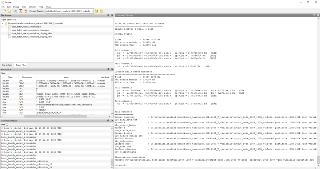
To show concretely the type of processing produced by the new version of the script, I used one of the series acquired today on the 100 Ω + 100 Ω divider with variable Vgen. The campaign includes 30 frequencies and, for each point, the two A and B acquisitions; the script works on the complete CSV files, with a three-component harmonic fit and the convention CH1 = VSENSE, CH2 = VOUT.
I do not yet want to use this series to draw definitive conclusions about the behavior of the test bench: some of the acquisitions were made before I identified the BNC connector problem described at the beginning of the article. At this stage I am mainly interested in using it to show what the program produces automatically.
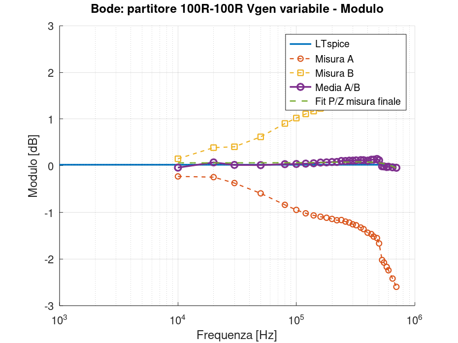
The first output is the standard magnitude plot. Measurement A and measurement B, the LTspice reference, their final combination, and the pole/zero fit are shown separately. The two transformer orientations clearly show errors of opposite sign, while the curve resulting from the A/B combination remains much closer to the reference. For example, between 50 and 120 kHz the final result remains between approximately 0.01 and 0.04 dB.
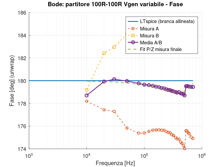
The same occurs in the phase plot, where A, B, the compensated average, LTspice, and the model obtained from the rational fit are displayed. Here too, the purpose of the figure is not yet to assess the test bench quantitatively, but to verify immediately the behavior of the two acquisitions and the result produced by the compensation.
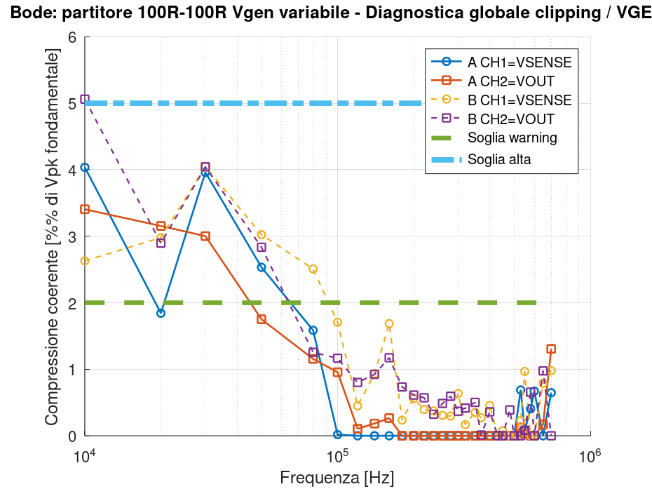
The third plot is instead dedicated to the new global deformation diagnostics. For each of the two channels, in configurations A and B, the coherent compression index calculated by the script is shown. The two horizontal lines indicate the thresholds currently set at 2% for a warning and 5% for severe deformation.
This diagnostic is not based on observing a single peak: the program folds many cycles onto the same phase, uses the median, and requires the deformation to be coherent over an extended region of the waveform. The report therefore distinguishes cases of possible compression from conditions in which the residual may be high but lacks a coherent structure, a situation more consistent with noise or spurious components.
This is exactly the kind of check I want for the next campaigns: not only to obtain magnitude and phase automatically, but also to have, together with the measurement, the information needed to understand how much I can trust the acquired point and under what conditions it was obtained.