GX-TXT-v3: Effect of Pulse Count on the HOLD Node Response

The GX-TXT-v3 is a circuit designed to provide a simple and immediate way to check the operation of infrared remote controls. The signal collected by the photodiode is amplified by a transistor chain and used to charge the HOLD node, which retains the received information for a certain time and drives the indicator LED.

The circuit therefore does more than simply detect the presence of IR radiation: the final response also depends on the intensity of the received signal, the gain and sensitivity control settings, and the timing structure of the pulse train.

The circuit schematic, operating principle, and PCB construction are described in the first article dedicated to the GX-TXT-v3:

GX-TXT-v3: IR Remote Control Tester – Circuit Schematic and Assembly

Final test with the virtual photodiode: effect of the number of pulses

As the final characterization of the GX-TXT-v3 using the virtual photodiode, I wanted to verify the effect of the number of received pulses while keeping the signal level and the circuit settings constant.

In the previous tests I had mainly studied the effect of the equivalent photodiode current and the sensitivity setting. In this series, the variable parameter is instead the burst duration, expressed directly as the number of pulses of the 38 kHz carrier.

Measurement conditions

Parameter	Value
Frequency	38 kHz
VGEN	about 3.2 Vpp
VRSENSE	1.020 Vpp
ISENSE	about 20 µA
P_GAIN	495 Ω
P_SENS	5.060 kΩ
Number of pulses	20, 40, 60, 80, 100, 120, 140
Time base for slow acquisitions	200 ms/div

The voltage measured across RSENSE was kept at about 1.020 Vpp for all acquisitions, corresponding to an equivalent virtual-photodiode current of about 20 µA. In this way the stimulus level remains constant, and the observed differences can mainly be attributed to the different number of applied pulses.

A note on the generator burst mode

Before showing the acquisitions, it is useful to clarify a detail about the generator operation in burst mode that I had not described precisely enough in the previous article.

In the configuration used, during the burst the generator produces the programmed pulse train, while between one burst and the next the output is not necessarily brought to zero: it remains at the level determined by the DC offset set on the generator.

This is particularly important in my case. To prevent the circuit used as a virtual photodiode from receiving the negative portion of the square wave, I applied a positive offset to the signal. The same offset therefore remains present during the intervals between one burst and the next.

For this reason, in the current tests I no longer consider the nominal amplitude set on the generator alone to be sufficient: I also directly check the voltage across RSENSE, using it as the experimental reference for the actual current produced by the virtual photodiode.

The oscillogram simultaneously shows the signal produced by the generator and the voltage measured across RSENSE. The carrier is 38 kHz, while the RSENSE level was adjusted to about 1.020 Vpp and kept unchanged throughout the entire series.

Circuit response as the number of pulses changes

Keeping all other conditions unchanged, I repeated the measurement with bursts of 20, 40, 60, 80, 100, 120, and 140 pulses. For each condition I acquired the HOLD node and the N_LED_ARANCIO node, also saving the complete traces in CSV format for subsequent numerical processing.

The following gallery directly shows the evolution of the circuit response. With 20, 40, and 60 pulses, HOLD is progressively charged, but the LED remains off. At 80 pulses the first clearly recognized turn-on appears, while further increasing the burst duration also increases the time for which the LED remains on.

Numerical processing of the acquisitions

For each test I also saved the complete oscilloscope traces in CSV format. With a sampling rate of 1.25 MSa/s, each file occupies several tens of megabytes, so it would make little sense to include the entire set of acquisitions directly in the article.

The CSV files were instead processed with GNU Octave using two scripts derived from those already developed for the previous GX-TXT-v3 measurements. The analysis structure remained essentially the same, but the batch process was adapted to the new test by adding the measured RSENSE voltage and the burst pulse count to the metadata.

For these acquisitions, the CSV contains only two oscilloscope channels: CH3, connected to the N_LED_ARANCIO node, and CH4, connected to the HOLD node. The script reconstructs the time axis from the data in the Rigol file header and automatically derives, among other quantities, the maximum value reached by HOLD and the LED on-time.

Automatic processing of individual acquisitions

The first script, GXTXT_batch_impulsi_v8_CH3_CH4.m, automatically analyzes all acquisitions listed in an index file. For each test it saves the numerical results, metadata, several intermediate tables, and graphs related to the dynamics of HOLD and the LED.

The index file contains one row for each acquisition and uses the following structure:

p_gain,p_sens,vgen_vpp,v_rsense_vpp,n_impulsi,nome_file_csv
495,5060,3.20,1.020,20,time_led_N020.csv
495,5060,3.20,1.020,40,time_led_N040.csv
...

The equivalent virtual-photodiode current is automatically derived from the voltage measured across the 51 kΩ RSENSE resistor:

I_SENSE ≈ V_RSENSE / 51 kΩ

To use the script, simply place the CSV files in the working folder, fill in the file prove_impulsi.csv with the actual measured values, and run:

GXTXT_batch_impulsi_v8_CH3_CH4

At the end, a batch folder is automatically created containing the results of the individual tests and the summary file risultati_batch.csv.

Global analysis of the series

The second script, GXTXT_analisi_impulsi_v1.m, uses the file risultati_batch.csv produced by the first script and combines all acquisitions into a single analysis. In particular, it generates the two graphs used in this article:

• maximum HOLD value as a function of the number of pulses;
• LED on-time as a function of the number of pulses.

Before running it, simply specify in the script the name of the batch folder just generated and then run:

GXTXT_analisi_impulsi_v1

The script also produces a CSV file and a text summary of the results, retaining as valid values the conditions in which the LED does not turn on, represented by T_LED = 0.

Download the scripts

The scripts used for this processing are available here:

Measurement series results

The seven acquisitions were performed while keeping the virtual-photodiode signal level and the GX-TXT-v3 settings constant, changing only the number of pulses in the burst.

The voltage across RSENSE remained at about 1.020 Vpp, corresponding to an I_SENSE of about 20 µA. This makes it possible to directly observe how the pulse-train duration affects the charge reached by the HOLD node and, subsequently, the LED on-time.

Number of pulses	Burst duration	VHOLD,max	TLED
20	0.5263 ms	0.44 V	LED off
40	1.0526 ms	0.96 V	LED off
60	1.5789 ms	1.28 V	LED off
80	2.1053 ms	1.56 V	0.5005 s
100	2.6316 ms	1.68 V	0.7065 s
120	3.1579 ms	1.84 V	0.8595 s
140	3.6842 ms	2.00 V	0.9725 s

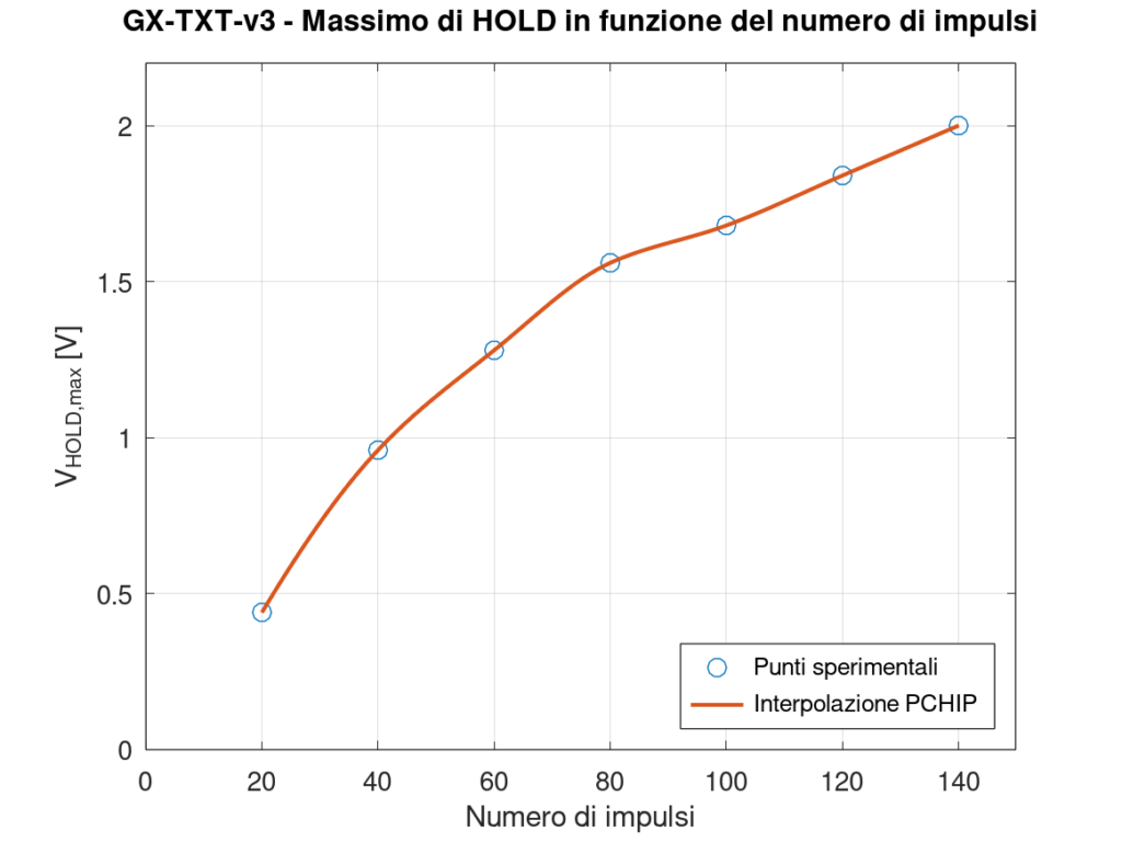
The first clear result is the progressive increase in the maximum value reached by HOLD as the number of pulses increases. With 20 pulses the node reaches only about 0.44 V; with 60 pulses it already reaches about 1.28 V, while with the longest burst, consisting of 140 pulses, it reaches about 2.00 V.

Maximum HOLD value as a function of the number of pulses

The first graph collects the V_HOLD,max values automatically derived from the CSV acquisitions. The growth is not perfectly linear: as the number of pulses increases, HOLD continues to charge, but the increment obtained with each additional group of pulses tends to decrease.

The line connecting the points is a simple PCHIP interpolation used as a visual guide and does not represent a physical model or a fit of the circuit behavior.

LED on-time

The effect on the indication time is even more evident. With 20, 40, and 60 pulses, the HOLD node is charged, but the level reached is not sufficient to turn on the LED. Under these conditions T_LED = 0 therefore represents a real experimental result, not missing data.

The first recognized turn-on in the series appears with 80 pulses: V_HOLD,max reaches about 1.56 V and the LED remains on for about 0.50 s. With 100 pulses the time rises to about 0.71 s, with 120 pulses to about 0.86 s, and with 140 pulses it reaches about 0.97 s.

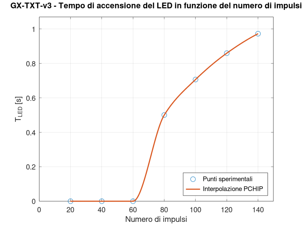
With the settings used in this test, the transition between no LED turn-on and LED turn-on therefore lies between 60 and 80 pulses. This is not a precise measurement of the threshold in terms of pulse count, but it experimentally identifies the relevant region.

Overall, the measurement shows the operating sequence of the circuit very clearly: as the burst duration increases, the level reached by HOLD rises and, once the region required to activate the output stage is exceeded, the time for which the LED remains on also increases.

Comparison with the relationship derived from previous measurements

There is an additional comparison that links this new series to the measurements performed previously. In the article devoted to HOLD dynamics, using different stimulus conditions, I had experimentally derived the relationship:

T_LED = 1.890 · ln(V_HOLD,max / 1.194)

This relationship was not derived using the data from the current test. It can therefore be used as an independent prediction of the LED on-time simply by inserting the V_HOLD,max values measured in the new variable-pulse-count series.

Number of pulses	VHOLD,max	TLED predicted	TLED measured
80	1.56 V	0.505 s	0.5005 s
100	1.68 V	0.645 s	0.7065 s
120	1.84 V	0.817 s	0.8595 s
140	2.00 V	0.975 s	0.9725 s

The agreement becomes even more significant when considering the resolution with which V_HOLD,max was determined. In the acquisitions used for this series, the exported HOLD values are quantized in steps of about 40 mV. Since the relationship used to predict T_LED depends logarithmically on V_HOLD,max, a single vertical step corresponds, in the region between about 1.5 and 2 V, to a predicted time variation on the order of 40–50 ms.

The maximum difference observed between prediction and measurement is about 61 ms, while at the other points it is smaller and at the ends of the series it falls to only a few milliseconds. It is important to emphasize that this is not a new fit of the data: the relationship was obtained from a previous measurement campaign, while here it is applied to a new series in which a different parameter—the number of pulses—was varied.

This result reinforces the interpretation of the circuit operation: once a given V_HOLD,max has been reached, the subsequent LED on-time depends mainly on the dynamics of the HOLD node, regardless of how that level was reached. Photodiode current, sensitivity setting, and number of pulses therefore affect the charging phase; the level reached by HOLD instead provides the link to the duration of the subsequent indication.

Comparison with LTspice simulation

The response to the number of pulses had also been studied in LTspice before the measurements on the real circuit. To make the comparison as consistent as possible with this new experimental test, the simulation used R_GAIN = 500 Ω and R_SENS = 5 kΩ, values very close to the 495 Ω and 5.060 kΩ used on the PCB.

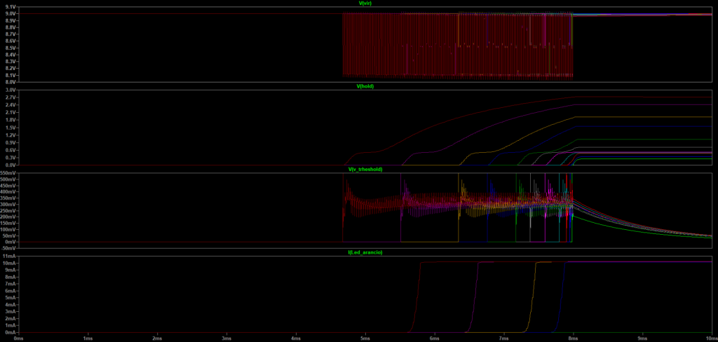
The simulation uses a sweep of the number of burst cycles and makes it possible to observe simultaneously the applied signal, the charging of the HOLD node, the V_THRESHOLD node, and the current through the orange LED. As the number of pulses increases, HOLD is also progressively charged in the simulation until it reaches the level required to activate the output stage.

Under the simulated conditions, with 32 pulses the LED is still off, while with 48 pulses a current of about 10 mA is already present. The transition predicted by the model therefore lies between 32 and 48 pulses. In the measurements on the real PCB, performed with I_SENSE ≈ 20 µA, the LED instead remains off up to 60 pulses and the first clearly recognized turn-on appears at 80 pulses.

The comparison becomes particularly interesting when looking at the HOLD node. In the simulation, with 48 pulses V_HOLD reaches about 1.56 V; in the real measurement, the first turn-on observed at 80 pulses likewise corresponds to a V_HOLD,max of about 1.56 V.

Condition	LTspice simulation	Real PCB
RGAIN	500 Ω	495 Ω
RSENS	5 kΩ	5.060 kΩ
ISENSE	20 µA	about 20 µA
Last point with LED off	32 pulses	60 pulses
First point with LED on	48 pulses	80 pulses
VHOLD at first LED-on point	about 1.56 V	about 1.56 V

The number of pulses required to obtain turn-on therefore does not match between the simulation and the real circuit. The HOLD value associated with activation is instead remarkably close. This suggests that an important part of the difference is related to how the model and the real circuit transfer and accumulate the charge produced by individual pulses, rather than to the behavior of the final stage once a given HOLD level has been reached.

I therefore do not consider the comparison a quantitative verification of the threshold expressed as a number of pulses, but rather a verification of the overall circuit dynamics. From this point of view, the simulation reproduces the experimentally observed behavior well: as the number of pulses increases, the HOLD voltage rises and, after a certain region is exceeded, the LED is activated.

It is significant that the first LED-on point in the simulation, at 48 pulses, and the first LED-on point observed on the PCB, at 80 pulses, both correspond to a HOLD value of about 1.56 V. The model and the real circuit therefore differ in the rate at which HOLD is charged by the pulse train, while they are much closer when the comparison is made directly at the level reached by the HOLD node.

Conclusions

This final series of tests with the virtual photodiode confirms that, with all other conditions unchanged, the maximum level reached by the HOLD node also depends on the number of received pulses:

V_HOLD,max = f(N_pulses)

The LED on-time therefore depends indirectly on the number of pulses through the level reached by HOLD. A longer burst charges the node to a higher level and, once the region required to activate the output stage has been exceeded, increases the time for which the LED remains on.

The P_SENS setting in turn changes the level reached by HOLD for the same received signal. The sensitivity potentiometer therefore controls not so much the brightness of the indicator LED, but whether the LED turns on and, when it does, how long the indication remains visible.

This behavior can be used in practice to compare different remote controls while keeping distance, orientation, and circuit settings constant. Using a reference remote control, it is possible to set a short and repeatable response and then observe how the indication changes when a second transmitter is used.

The same principle also suggests a possible direction for future development. The relationship between the received optical signal, the circuit response, and the voltage reached by HOLD could provide the basis for an instrument dedicated to the quantitative characterization of IR LEDs and transmitters.

However, measuring optical power would require an instrument designed specifically for that purpose, with defined measurement geometry, shielding from ambient light, controlled distance, an adjustable aperture or slit, a properly characterized photodiode, and calibration references. It would therefore be a separate and significantly more complex project than the GX-TXT-v3.

The most natural next step will therefore be to stop using the virtual photodiode and repeat the characterization with one or more real photodiodes. This will make it possible to directly observe the signal produced by an IR remote control, study its carrier and bursts at the VINPUT node, and verify how the behavior measured so far with a controlled stimulus transfers to real operating conditions.