Lesson 07 — Creating and Publishing Scientific Datasets

From numerical vectors to reusable scientific data: sine waves, metadata, public APIs, and atomic publication.

In previous lessons, we learned to write GNU Octave programs, recognize GX-TXT Datasets, and read their variables through stable identifiers. We will now go in the opposite direction: starting with a mathematical model, we generate values in Octave and publish the results as canonical GX-TXT Datasets.

This introduces an important concept in scientific programming: producing an array of numbers is not the same as producing a Dataset. A Dataset also contains information about what those numbers represent, their units, provenance, and variable structure. GX-TXT also handles registration and storage management.

We will carry out two exercises in sequence:

1. A voltage sine wave with an offset, published as a single Dataset.
2. Three related signals — pure, noisy, and with a third harmonic — published in one atomic transaction.

The examples are entirely synthetic, so no measurements or input files are needed. The scripts contain English comments, and this article explains how they work.

1. What Is New Compared with Previous Lessons

Lessons 01–04 introduced variables, operators, vectors, matrices, loops, and functions. Lesson 05 focused on Dataset identities and Variable IDs, while Lesson 06 showed how to read scientific data using the public APIs.

In this lesson, we will not repeat the syntax already covered from the beginning: instead, we will apply it to build something new.

Concept	Previously covered	New in this lesson
Vectors	Creating vectors and numerical operations	Rigorous construction of a sampled time axis
Elementwise operations	Octave operators and functions	Generating physically interpretable signals
for and if	Flow control	Systematically building publication requests and checks
struct	Reading metadata	Building scientific descriptors and nested requests
Cell arrays	Collections and Bridge arguments	Collecting several publication requests into a batch
Dataset ID and Variable ID	Identity and inspection	Choosing IDs for new scientific results
Reading Datasets	Canonical APIs	Verifying new results and distinguishing reading from writing
Numerical processing	Native Octave functions	Comparing them with public NUMERIC_API_v1 operations
Publication	Not yet covered	publish_series, publish_series_batch, and atomicity

The central question is: how can we turn computed values into scientifically described results that are available within the Session?

2. What Does It Mean to Publish a Dataset?

Consider two vectors:

time_s = [0; 0.1; 0.2; 0.3];
voltage_v = [0; 1; 0; -1];

In memory, Octave holds four numbers for each variable. Their names suggest that these represent time and voltage, but the suffixes _s and _v do not automatically enable a physical-unit system.

A scientific Dataset must explicitly declare at least the information needed to interpret its numbers. In our examples, its logical structure will be:

Dataset: lesson07_sine_clean
│
├── Variable ID: time_s
│   ├── Name: time_s
│   ├── Display label: Elapsed time
│   ├── Unit: s
│   ├── Data type: float64
│   └── Semantic role: time
│
├── Variable ID: voltage_v
│   ├── Name: voltage_v
│   ├── Display label: Simulated voltage
│   ├── Unit: V
│   ├── Data type: float64
│   └── Semantic role: voltage
│
└── Structured metadata
    ├── Model
    ├── Frequency
    ├── Amplitude
    ├── Offset
    └── Sample rate

We already encountered the Dataset ID + Variable ID pair in Lesson 05. Now we will learn to define it ourselves.

A Dataset ID is not a filename, and a Variable ID is not a CSV column number. This separation allows the framework to use different storage backends, such as CSV or HDF5, without changing the scientific meaning of these identifiers.

3. First Experiment: A Sine Wave with DC Offset

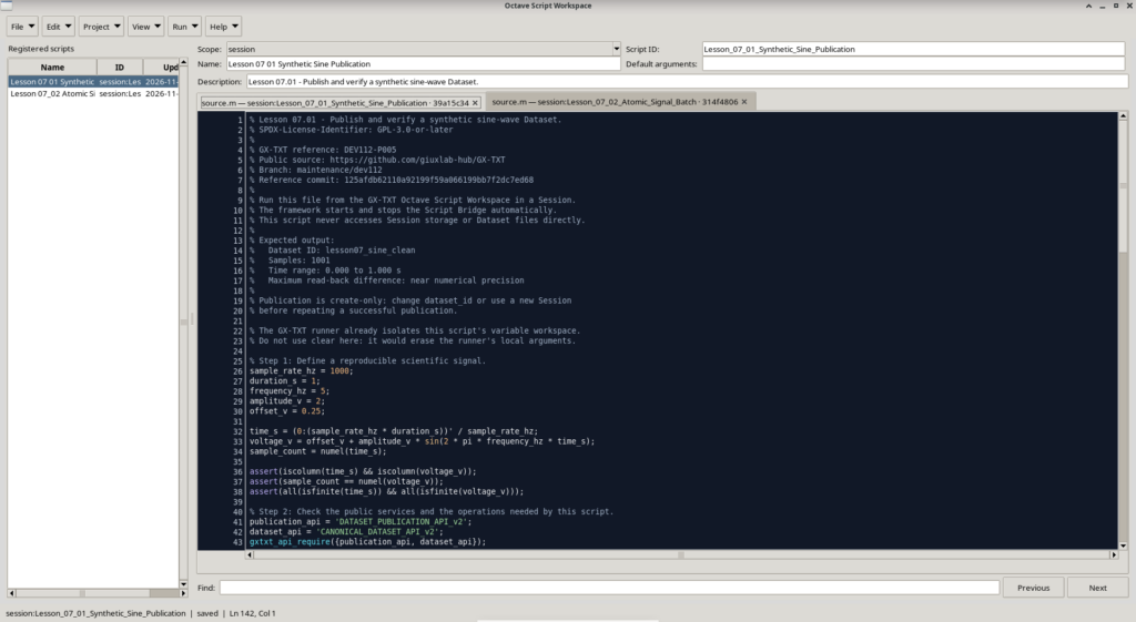
The Lesson_07_01_Synthetic_Sine_Publication.m script generates a voltage defined by:

The parameters are:

Quantity	Symbol	Value
Voltage offset	\(U_0\)	0.25 V
Peak amplitude	\(A\)	2 V
Signal frequency	\(f\)	5 Hz
Sampling frequency	\(f_s\)	1000 Hz
Duration	\(T\)	1 s

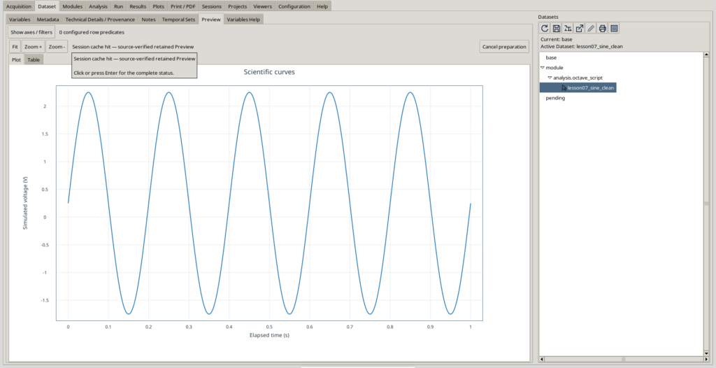
The resulting sine wave has a minimum of −1.75 V and a maximum of +2.25 V.

3.1 Parameters: Assignment, Names, and Units

sample_rate_hz = 1000;
duration_s = 1;
frequency_hz = 5;
amplitude_v = 2;
offset_v = 0.25;

Each statement assigns a numerical value to a variable. The semicolon suppresses automatic output, allowing the program to print only a meaningful summary when it finishes.

The signal frequency must not be confused with the sampling frequency. The former tells us how many oscillations occur per second; the latter tells us how many values we calculate over the same interval.

At 5 Hz, the period is:

At a sampling rate of 1,000 Hz, one period is represented by 200 sampling intervals. The Nyquist frequency is 500 Hz, well above the signal frequency. This does not guarantee accuracy for every possible signal, but it explains why our sine wave is sampled at adequate resolution.

3.2 The Time Axis: Understanding the : Operator

time_s = (0:(sample_rate_hz * duration_s))' / sample_rate_hz;

This line deserves to be read in full rather than copied mechanically.

1. Compute the final index. The product sample_rate_hz * duration_s equals 1000.

2. Generate the indices. 0:1000 generates integers from 0 through 1000, including both endpoints. The result has 1,001 elements.

3. Transpose. The apostrophe ' turns a row vector into a column vector. For real-valued data, conjugate transpose is equivalent to ordinary transpose; for complex-valued data, ' and .' are not interchangeable.

4. Convert to seconds. Each index is divided by the sampling frequency:

The time step is \(\Delta t=1/f_s=0.001\,\mathrm{s}\). The endpoints are 0 and 1 s.

Why do we get 1,001 samples rather than 1,000? Because we include both the start and end points. When \(f_sT\) is an integer, the number of points is \(N=f_sT+1\). Other experiments may use a grid that excludes the final endpoint. That is not an error; it is a different sampling convention.

3.3 Vectorized Calculation: One Function Applied to Many Values

voltage_v = offset_v + amplitude_v * ...
            sin(2 * pi * frequency_hz * time_s);
sample_count = numel(time_s);

GNU Octave’s sin() function is applied to every element of the vector. There is no need for a loop that computes one voltage at a time.

For each element \(t_k\), the phase \(2\pi f t_k\) is formed first, then its sine is computed, multiplied by the amplitude, and finally shifted by the offset.

Notice that the sine function receives a phase expressed in radians, a dimensionless quantity. It does not receive seconds or hertz directly: their product yields the correct argument.

The numel() function returns the total number of elements. This differs from length(), which returns the largest dimension, and size(), which describes the shape of the array. The distinction is straightforward for a column vector but becomes important for matrices and multidimensional arrays.

3.4 Checks Before Publication

assert(iscolumn(time_s) && iscolumn(voltage_v));
assert(sample_count == numel(voltage_v));
assert(all(isfinite(time_s)) && all(isfinite(voltage_v)));

Three properties are checked before publication:

• Shape: both arrays must be column vectors.
• Consistency: the time and voltage vectors must have the same number of samples.
• Numerical validity: every value must be finite, neither NaN nor infinity.

The && operator is the logical AND of scalar conditions. all(isfinite(...)) reduces the checks on all elements to a single logical result.

assert() stops execution when a condition is not met. It is better to detect a data problem before asking the framework to publish the values.

4. Numerical Functions: Native Octave and GX-TXT Public APIs

The first script performs its calculations using sin() and GNU Octave’s native numerical operators. This is entirely normal: using GX-TXT does not mean giving up the Octave language.

However, the framework also provides a public numerical API, NUMERIC_API_v1, with operations on scalars, vectors, and matrices. It is useful to know this API while keeping it distinct from native functions.

4.1 Which GX-TXT Operations Correspond to Our Calculations?

Calculation	GNU Octave	GX-TXT API
Elementwise sine	sin(v)	array_unary with sin
Multiply by a scalar	v * A	array_binary with multiply
Add an offset	v + U0	array_binary with add
Minimum and maximum	min(v), max(v)	array_reduce with minimum, maximum
Mean value	mean(v)	array_reduce with mean
RMS value	sqrt(mean(v.^2))	array_reduce with rms

The names array_unary, array_binary, and array_reduce are operations of the numerical service, not private Tcl functions to be invoked directly.

4.2 How to Represent a Numerical Operand

The numerical API requires more than a raw number: when called through the Bridge, it uses a structure that declares the shape of the operand.

phase = 2 * pi * frequency_hz * time_s;

phase_operand = struct( ...
    'kind', 'vector', ...
    'value', phase);

The kind field distinguishes scalar, vector, and matrix. The value field holds the numerical data. This is an Octave structure, not a copy of a Dataset stored on disk.

We can represent a scalar in the same way:

gain_operand = struct('kind', 'scalar', 'value', amplitude_v);

This explicit description allows the API to check operand types, shapes, and compatibility. Binary operations can expand a scalar across a vector; two non-scalar arrays must have compatible shapes according to the operation’s contract.

4.3 array_unary: Computing the Sine with GX-TXT

gxtxt_api_require({'NUMERIC_API_v1'});

sine_result = gxtxt_api_call( ...
    'NUMERIC_API_v1', ...
    'array_unary', ...
    {'sin', phase_operand});

sine_values = sine_result.values;

Let us explain each component:

• gxtxt_api_require() checks that the required API is available in the execution context.
• gxtxt_api_call() is the general function of the Octave Script Bridge.
• 'NUMERIC_API_v1' identifies the public service being called.
• 'array_unary' identifies a single-operand operation.
• {'sin', phase_operand} is the cell array of positional arguments: the mathematical operation name and the operand descriptor.
• sine_result.values extracts the returned vector from the result structure.

Curly braces do not denote a numerical vector: they construct a cell array. This distinction, introduced in earlier lessons, is particularly important in the Bridge because the function receives an ordered collection of arguments.

4.4 array_binary: Amplitude and Offset

We can complete the sine wave using two public binary operations.

gain_result = gxtxt_api_call( ...
    'NUMERIC_API_v1', ...
    'array_binary', ...
    {'multiply', ...
     struct('kind', 'vector', 'value', sine_values), ...
     struct('kind', 'scalar', 'value', amplitude_v)});

voltage_result = gxtxt_api_call( ...
    'NUMERIC_API_v1', ...
    'array_binary', ...
    {'add', ...
     struct('kind', 'vector', 'value', gain_result.values), ...
     struct('kind', 'scalar', 'value', offset_v)});

voltage_from_gxtxt = voltage_result.values;

multiply performs elementwise multiplication, and add performs addition. Because one operand is a scalar and the other a vector, the scalar is applied to every vector element.

This example shows that we can obtain the same mathematical expression using either native Octave statements or NUMERIC_API_v1.

The main lesson scripts use native Octave functions to generate the signals. The calls shown here introduce the equivalent public numerical interface without changing the experiment.

4.5 array_reduce: From a Vector to a Summary Value

operand = struct('kind', 'vector', 'value', voltage_v);

minimum_result = gxtxt_api_call( ...
    'NUMERIC_API_v1', 'array_reduce', {'minimum', operand});

maximum_result = gxtxt_api_call( ...
    'NUMERIC_API_v1', 'array_reduce', {'maximum', operand});

rms_result = gxtxt_api_call( ...
    'NUMERIC_API_v1', 'array_reduce', {'rms', operand});

minimum_v = minimum_result.values;
maximum_v = maximum_result.values;
rms_v = rms_result.values;

A reduction turns a collection of samples into one or more summary values, depending on the requested axis and operation. For a simple vector, a global reduction produces a single value.

The RMS value is:

Do not confuse RMS with standard deviation. Our first signal has an offset: the DC component contributes to the RMS value but is not a fluctuation around the mean.

The array_unary, array_binary, and array_reduce operations do not automatically assign physical units to vectors and do not perform implicit unit conversions. The person constructing the calculation is responsible for dimensional consistency; units are explicitly declared in the variable descriptors during publication.

Non-finite values and results outside the real-number domain are also subject to the checks defined by the numerical API contract. This is one reason to understand public APIs beyond simply knowing that equivalent operations are available in Octave.

5. Declaring the Variable Schema

After computing the signal, we reach our first real publication task: telling GX-TXT what the vectors contain.

5.1 struct(): Creating a Scientific Descriptor

x_variable = struct( ...
    'variable_id', 'time_s', ...
    'name', 'time_s', ...
    'display_label', 'Elapsed time', ...
    'unit', 's', ...
    'dtype', 'float64', ...
    'value_kind', 'number', ...
    'semantic_role', 'time', ...
    'semantic_source', 'generator');

The struct() function creates a structure from pairs of field names and values. It resembles the records we read through the APIs in Lesson 05, but this time we create the descriptor ourselves.

Field	Meaning
variable_id	Stable identifier of the variable within the Dataset
name	Declared scientific name
display_label	Human-readable label
unit	Declared physical unit
dtype	Element type, here float64
value_kind	Kind of value, here number
semantic_role	Scientific meaning of the variable
semantic_source	Origin of the semantic declaration

dtype and value_kind are not synonyms. The former describes how a value is represented; the latter describes the kind of value it is. The publication contract accepts number, text, and elapsed_time for value_kind. In our case, time is already represented numerically in seconds, so number is appropriate. The elapsed_time value has a specific contract for HMS-formatted data.

semantic_source = 'generator' indicates that the semantic declaration comes from the generator. It does not claim that a measurement was performed, and it does not turn simulated numbers into acquired data.

The second variable follows the same pattern:

y_variable = struct( ...
    'variable_id', 'voltage_v', ...
    'name', 'voltage_v', ...
    'display_label', 'Simulated voltage', ...
    'unit', 'V', ...
    'dtype', 'float64', ...
    'value_kind', 'number', ...
    'semantic_role', 'voltage', ...
    'semantic_source', 'generator');

Notice that the time_s / voltage_v pair is understandable without knowing which software generated the signal.

5.2 Structured Metadata: Preserving the Calculation Context

metadata = struct();
metadata.('simulation.model') = 'offset sine wave';
metadata.('simulation.frequency_hz') = frequency_hz;
metadata.('simulation.amplitude_v') = amplitude_v;
metadata.('simulation.offset_v') = offset_v;
metadata.('simulation.sample_rate_hz') = sample_rate_hz;

The new syntax is metadata.('simulation.frequency_hz'): this accesses a field using a dynamic field name, written in parentheses and quotes.

We cannot write metadata.simulation.frequency_hz and expect the same result: that syntax would represent two levels of nested structures, whereas simulation.frequency_hz is one field name containing a period. This distinction matters when APIs and registries use qualified metadata keys.

These metadata are not decoration. They preserve the conditions needed to interpret and reproduce the model: frequency, amplitude, offset, and sampling rate.

A sine wave generated at 5 Hz and one generated at 50 Hz could contain the same number of samples. Without metadata, that distinction would be easy to lose.

6. Building the Publication Request

We now bring the data, descriptors, and metadata together in one Octave structure that will be passed to the public service.

request = struct( ...
    'dataset_id', dataset_id, ...
    'contract', 'table.generic', ...
    'storage', 'auto', ...
    'x_values', time_s, ...
    'y_values', voltage_v, ...
    'x_variable', x_variable, ...
    'y_variable', y_variable, ...
    'producer_version', '1.0.0', ...
    'source', 'GNU Octave synthetic signal generator', ...
    'provenance', 'Deterministic 5 Hz offset sine wave', ...
    'notes', 'GNU Octave with GX-TXT, Lesson 07.01', ...
    'structured_metadata', metadata);

Several new ideas appear here.

Nested structures. The x_variable and y_variable fields each contain another structure, and structured_metadata contains yet another. Octave can build this collection of information without requiring custom classes or serialization formats.

The table.generic contract. This declares the Dataset’s general tabular scientific contract. It is not a filename and does not directly require a particular physical storage backend.

storage = 'auto'. This asks GX-TXT to choose an appropriate storage backend according to its policy. The caller need not select a path or write CSV/HDF5 files manually.

Source and provenance. source, provenance, producer_version, and notes provide additional context. They differ from IDs: they describe the result rather than define its identity.

This is the difference between a program that saves two columns to a file and a program that publishes a scientific result managed by the framework.

7. The First Write API: publish_series

The central call in the first script is:

receipt = gxtxt_api_call( ...
    'DATASET_PUBLICATION_API_v2', ...
    'publish_series', ...
    {request});

7.1 Purpose and Syntax

Element	Role
DATASET_PUBLICATION_API_v2	Identifier of the public publication API
publish_series	Operation for publishing one-dimensional X/Y series
{request}	Cell array containing one positional argument, the request structure
receipt	Structure returned with the publication result

publish_series requires a dataset_id, a contract, two non-empty X/Y arrays of equal length, and two variable descriptors with distinct variable_id values.

The service handles preparation, variable declaration, writing, and finalization. The public components responsible for the Dataset validate the required conditions.

7.2 What Finalization Means

Publication is more than writing an array: it must produce a coherent Dataset. The framework manages the commit operation and registration in the Session catalog.

A failure during publication must prevent an incomplete new Dataset from remaining in the catalog. Following a successful publication, the Dataset becomes an actually registered resource.

The example normally uses create-only mode: if an ID already exists, we do not silently overwrite existing data.

This is why the script first checks the catalog:

existing_ids = gxtxt_api_call( ...
    'CANONICAL_DATASET_API_v2', 'list', {});

if any(strcmp(existing_ids, dataset_id))
  error('Dataset already exists');
endif

strcmp() compares strings, and any() checks whether at least one comparison is true. This preliminary check provides a clear message, while GX-TXT remains the ultimate authority on ID availability and publication.

7.3 What the Bridge Does

We have already used gxtxt_api_call() to read Datasets. Now the same function can invoke an authorized write operation.

The Bridge is not a general-purpose Tcl command executor, and it does not automatically expose every internal CORE method. A call is allowed only when the API and operation are registered for script use.

This is why the scripts begin with:

publication_api = 'DATASET_PUBLICATION_API_v2';
dataset_api = 'CANONICAL_DATASET_API_v2';

gxtxt_api_require({publication_api, dataset_api});

if !gxtxt_api_has_operation(publication_api, 'publish_series')
  error('Publication operation unavailable');
endif

gxtxt_api_require() declares the required services. gxtxt_api_has_operation() checks that the exact requested operation is available, not merely the API name.

8. Results of the First Experiment

The published Dataset has the ID lesson07_sine_clean. It contains 1,001 samples over the time interval from 0 to 1 second. Voltage ranges from −1.75 V to +2.25 V.

The original script also performs a canonical read using CANONICAL_DATASET_API_v2/read_range and compares the values with the original vectors. This operation revisits the method introduced in Lesson 06: read_range takes a Dataset ID, a cell array of Variable IDs, a zero-based start index, and the number of samples.

In everyday use, after publication we can simply open the Dataset in GX-TXT’s Dataset panel and use Preview to inspect the curve and metadata. There is no need to create a second script solely to display what the framework already provides.

9. Second Experiment: Three Synthetic Signals

With the second script, Lesson_07_02_Atomic_Signal_Batch.m, we apply what we have learned to create several Datasets in one operation.

We use a 5 Hz fundamental sine wave with an amplitude of 1.5 V, a duration of 2 s, and a sampling frequency of 400 Hz.

The axis contains \(400\times2+1=801\) points. The time step is 2.5 ms, and each 0.2 s period spans 80 sampling intervals.

9.1 The Three Mathematical Models

The pure sine wave is:

The second signal adds synthetic Gaussian noise:

The third adds a third harmonic:

The third harmonic has three times the fundamental frequency and 30% of its amplitude. It is not random noise: it is a deterministic component that systematically alters the waveform.

9.2 The Pseudorandom Generator: rng() and randn()

rng(707, 'twister');

pure_v = amplitude_v * ...
    sin(2 * pi * frequency_hz * time_s);

noisy_v = pure_v + ...
    noise_standard_deviation_v * randn(sample_count, 1);

randn(sample_count, 1) generates a column vector of pseudorandom samples from a standard normal distribution, which has theoretical mean zero and theoretical standard deviation one. Multiplying by 0.2 scales the theoretical standard deviation to 0.2 V.

The number 707 is the generator’s seed. rng(707, 'twister') sets the initial state of a particular pseudorandom generator family. By fixing the algorithm, seed, and a compatible computing environment, the sequence can be reproduced. This improves reproducibility of the model; it does not simulate the properties of any particular oscilloscope.

A finite noise realization will not necessarily have a sample mean of exactly zero or a measured standard deviation of exactly 0.2 V. These are the parameters of the distribution used to generate the data.

Is there an equivalent GX-TXT function? The framework offers several public numerical operations, including reductions and resampling primitives, but resampling indices must not be confused with generating an independent normally distributed noise vector. In this exercise, the native Octave function randn() is appropriate; NUMERIC_API_v1 remains available for further vector analysis.

9.3 The Third Harmonic and Vector Operations

harmonic_v = pure_v + ...
    third_harmonic_amplitude_v * ...
    sin(2 * pi * (3 * frequency_hz) * time_s);

We are adding two vectors of the same size. The first is the fundamental; the second is the 15 Hz harmonic.

This also illustrates another principle: signals that share the same time axis can be compared sample by sample. We should not directly add samples from incompatible time grids without first defining an explicit alignment or resampling rule.

10. A New Application of Cell Arrays

signal_values = {pure_v, noisy_v, harmonic_v};

dataset_ids = {'lesson07_sine_pure', ...
               'lesson07_sine_noisy', ...
               'lesson07_sine_harmonic'};

We have two parallel cell arrays:

• signal_values holds three numerical vectors.
• dataset_ids holds three text identifiers.

The first element of each corresponds to the pure sine wave, the second to the noisy one, and the third to the harmonic signal.

To access the contents of a cell, we use curly braces:

first_signal = signal_values{1};
first_id = dataset_ids{1};

signal_values(1), by contrast, would return a cell array containing one cell. This distinction is essential when passing its contents into a publication request.

10.1 Preallocation and the Construction Loop

series_requests = cell(1, numel(dataset_ids));

for k = 1:numel(dataset_ids)
  metadata = struct();
  metadata.('simulation.model') = model_labels{k};

  series_requests{k} = struct( ...
      'dataset_id', dataset_ids{k}, ...
      'contract', 'table.generic', ...
      'storage', 'auto', ...
      'x_values', time_s, ...
      'y_values', signal_values{k}, ...
      'x_variable', time_variable, ...
      'y_variable', voltage_variable, ...
      'structured_metadata', metadata);
endfor

This block is an abbreviated version of the full script, which also includes further provenance fields and model parameters.

Preallocating with cell(1, numel(dataset_ids)) reserves a collection of three cells before the loop. At each index k, the program constructs the publication structure for the corresponding signal.

The loop is not intended to replace vectorized numerical computation: instead, it creates three similar but distinct structured descriptors, for which a loop is a natural choice.

Each structure includes:

• A different Dataset ID.
• A shared time axis.
• A different voltage vector.
• The same internal IDs, time_s and voltage_v, which are valid within each distinct Dataset.
• Metadata specific to the model.

Two distinct Datasets may both contain a variable called voltage_v: pairing it with the Dataset ID makes the identity unique.

11. Atomic Publication: publish_series_batch

This is the major new concept in the second experiment.

We could call publish_series three times. If the first and second publications succeeded but the third failed, we would be left with two new Datasets but not the third. That would no longer be the complete set of results we intended to publish.

GX-TXT addresses this situation with publish_series_batch, which coordinates a create-only publication of multiple X/Y series within one transaction.

11.1 Preparing the Request

batch_request = struct();
batch_request.series = series_requests;

The structure has just one field, series, containing the cell array of three requests prepared earlier.

11.2 Calling the Framework

receipt = gxtxt_api_call( ...
    'DATASET_PUBLICATION_API_v2', ...
    'publish_series_batch', ...
    {batch_request});

The API receives a single positional argument: the batch_request structure.

The receipt contains information such as:

Field	Meaning
atomic	Confirms the atomic nature of publication
output_count	Number of Datasets produced
dataset_ids	Identifiers of the outputs
datasets	Receipts for individual Dataset publications

The script checks the receipt:

if !receipt.atomic || ...
   receipt.output_count != numel(dataset_ids)
  error('Unexpected batch publication result');
endif

The ! operator denotes logical negation, and || is logical OR. The condition raises an error if the receipt does not confirm the requested result.

11.3 What Atomicity Means

An atomic transaction follows the all-or-nothing principle: the new outputs belong to the same publication operation. GX-TXT, not the Octave script, is responsible for commits and any rollback.

In our case, the result is a set of three separate Datasets, not one Dataset with three columns and not automatically a Dataset Group. Keep this distinction in mind when inspecting the results within the Session.

The contract prevents accidental overwriting: a create-only batch that encounters an already registered ID is rejected. To repeat the experiment and publish additional results, use new IDs or a new Session.

This API is particularly useful when results have a shared meaning, for example three experimental conditions, several replicates, or signals processed during the same simulation.

12. Interpreting the Three Previews

The second exercise publishes three Datasets, each with 801 samples and two variables.

Dataset ID	Signal	Main characteristic
lesson07_sine_pure	5 Hz sine wave	Regular periodic waveform
lesson07_sine_noisy	Sine wave plus normal noise	Random fluctuations around the fundamental
lesson07_sine_harmonic	Fundamental plus third harmonic	Deterministic periodic distortion

The Preview of the pure signal shows a regular waveform. The noisy curve is perturbed by pseudorandom samples. The third signal, although completely deterministic, is no longer a simple sine wave because two frequencies have been combined.

These are three different mathematical phenomena: ideal signal, random perturbation, and harmonic distortion. We should not describe every difference generically as “noise.”

1 / 3

Open the full gallery page Download gallery ZIP (HTML + hi-res images)

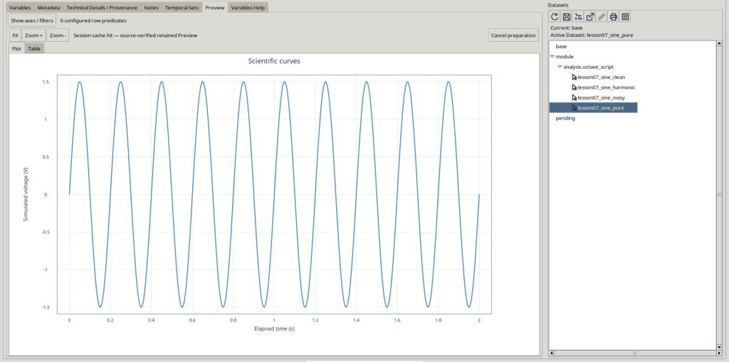
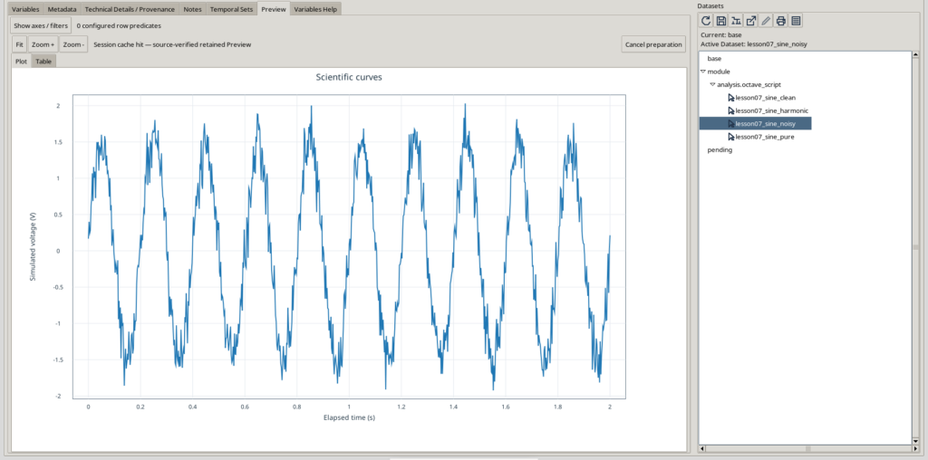
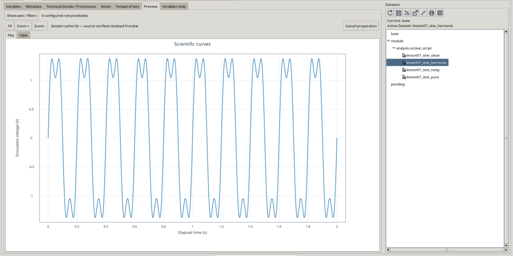
Three synthetic signals published atomically as separate Datasets. The time axis and variable schema are shared; the mathematical model of the voltage differs.

Preview is a tool for inspecting data that have already been published. In this lesson, we do not generate images using Octave’s native plotting functions. The next lesson will cover scientific visualization and structured plotting through the public GX-TXT Plot Dataset APIs.

13. Summary of the Public APIs Used and Available

It is useful to distinguish three groups of APIs:

A. Octave Script Bridge API v1

Function	Arguments	Purpose
gxtxt_api_require()	Cell array of requirements	Checks the required public dependencies
gxtxt_api_has_operation()	API ID and operation name	Checks availability of a specific operation
gxtxt_api_call()	API ID, operation, cell array of arguments	Invokes a registered public operation

The Bridge is the common entry point. User code should not start or stop it manually: GX-TXT manages the execution lifecycle.

B. Dataset Publication API v2 and Canonical Dataset API v2

API / operation	Purpose
DATASET_PUBLICATION_API_v2 / publish_series	Publishes one X/Y series with schema and metadata
DATASET_PUBLICATION_API_v2 / publish_series_batch	Atomically publishes multiple X/Y series as separate Datasets
CANONICAL_DATASET_API_v2 / list	Lists Dataset IDs in the Session
CANONICAL_DATASET_API_v2 / describe	Returns the Dataset description and variables
CANONICAL_DATASET_API_v2 / read_range	Reads a range of values using Variable IDs and logical indices

C. Numeric API v1

Operation	Purpose
array_unary	Transforms an array by applying, for example, sine or square root
array_binary	Combines two operands through additions, products, and other operations
array_reduce	Computes descriptive statistics and summary values

The examples in Section 4 show how the public Numeric API can also perform calculations that the main scripts carry out with native Octave. Which approach to choose depends on the objective: learning the language, using shared numerical contracts in the framework, or composing more complex analyses.

One principle remains unchanged: Dataset access and publication must use the framework’s canonical APIs, without manipulating the internal Session files.

14. Exercises to Try on Your Own

Once you understand the two scripts, modify their parameters and predict the results before running them.

1. Frequency and number of cycles. In the first experiment, change frequency_hz from 5 to 8 without changing the sampling rate or duration. How many cycles appear between 0 and 1 s? Does the number of samples change? Why?
2. Offset. Replace offset_v = 0.25 with offset_v = -1. Determine the theoretical minimum, maximum, and mean of the sine wave before publication.
3. Sampling. In the second script, increase sample_rate_hz to 800 Hz. How many samples are generated in 2 s? What changes in the Preview, and what remains physically unchanged?
4. Noise. Change the nominal standard deviation from 0.20 V to 0.05 V. With the same seed, what relationship remains between the noise sequences? How does the signal-to-noise ratio change?
5. Harmonics. Set the third-harmonic amplitude first to zero and then to 0.75 V. What is the difference between harmonic distortion and random perturbation?
6. Structures. Add a simulation.duration_s metadata field to all batch requests. Identify the most appropriate place in the loop to do this.
7. Numerical APIs. Use NUMERIC_API_v1 / array_reduce to compute the minimum, maximum, and RMS of all three vectors. Compare the results with min(), max(), and the native expression sqrt(mean(v.^2)).

Each variant that you intend to publish must use new Dataset IDs or a dedicated Session. Do not overwrite previous results just because you have modified a script.

15. What We Have Learned

This lesson brings together the two sides of our course: GNU Octave as a computational language and GX-TXT as a scientific data infrastructure.

We have seen how to build a time axis, apply a mathematical function to an entire vector, understand why the number of samples depends on the included endpoints, and introduce reproducible random components.

We then used Octave structures to describe variables and metadata, carefully distinguishing identities, labels, units, and data types. Finally, we entrusted publication to DATASET_PUBLICATION_API_v2, first for a single signal and then for three atomic outputs.

The result is not simply a curve drawn on a screen. It consists of scientific Datasets that GX-TXT can identify, describe, and make available to other tools.

The next lesson will explore scientific visualization in more depth, distinguishing a simple Preview from a structured representation managed through the public Plot Dataset APIs.

Lesson Materials

The GNU Octave scripts associated with this article are:

• Lesson_07_01_Synthetic_Sine_Publication.m — generates a sine wave with an offset and publishes it as a canonical Dataset.
• Lesson_07_02_Atomic_Signal_Batch.m — generates three synthetic signals and publishes them in one atomic transaction.

Both scripts use native Octave functions to generate numerical data and GX-TXT public APIs to publish Datasets. They are distributed under the GNU GPL v3 or later.

Reference Version and Documentation

This lesson refers to GX-TXT DEV112-P005 and the public API contracts in the GX-TXT GitHub repository, branch maintenance/dev112, commit 125afdb62110a92199f59a066199bb7f2dc7ed68.

For more information about the interfaces used:

• Octave Script Bridge API v1
• Dataset Publication API v2
• Canonical Dataset API v2
• Dataset Variable Schema API v3
• Numeric API v1