

Lesson 10 – Interpolation and Fitting: An Analytical Calibration Curve
Scientific programming course with GNU Octave and the GX-TXT public APIs.
In the previous lessons, we learned to work with Datasets, visualize scientific results and calculate descriptive statistics. In this lesson, we will use data to build a mathematical model: starting from nine synthetic calibration standards, we will compare interpolation and regression, examine residuals and determine the concentration of an unknown sample.
Connections with the previous lessons
Lessons 05–07 introduced Dataset IDs, Variable IDs and result publication; Lesson 08 covered persistent plots and the debugger; Lesson 09 explained descriptive statistics. Now, rather than merely describing our data, we estimate a mathematical relationship and evaluate its predictive ability. We will use sort(), RMS and canonical Datasets again, but apply them to a new problem.
The main new concepts are linspace(), polyval(), least-squares regression, interpolation, model residuals and the public operations linear_regression, interpolate and polynomial_fit.
The learning path also includes a deliberate error and its diagnosis with the native GNU Octave debugger. Results will be published as GX-TXT Datasets and persistent plots, without accessing the framework’s internal files.
Prerequisites: knowledge from Lessons 05–09, or familiarity with Octave vectors and functions, Dataset IDs, Variable IDs and the Octave Script Workspace. To repeat the complete exercise, create a fresh GX-TXT Session: the scripts publish Datasets with explicit identifiers and do not overwrite existing ones.
Important: all concentration and absorbance values are synthetic and deterministic, created for teaching purposes. They are not experimental measurements, certified standards or analytical-method validation data.
1. Learning objectives
By the end of the lesson, we will be able to distinguish interpolation from fitting, correctly sort paired observations, perform linear least-squares regression, compare it with a second-degree polynomial, interpret residuals and the coefficient of determination, estimate an unknown concentration within the calibration range, and use the GX-TXT public APIs to preserve and visualize the results.
2. Our experiment: concentration and absorbance
Consider an optical measurement described by the absorbance \(A\) of solutions with known concentration \(C\), expressed in mg/L. Within the selected range, we expect an approximately linear relationship:
\[A = a + bC + \varepsilon\]
Here \(a\) is the intercept, \(b\) is the slope, and \(\varepsilon\) represents the part of the signal not explained by the model. We do not assume a perfect straight line: its coefficients must be estimated from the data.
| Concentration \(C\) (mg/L) | Synthetic absorbance \(A\) |
|---|---|
| 0 | 0.010 |
| 1 | 0.096 |
| 2 | 0.177 |
| 3 | 0.258 |
| 4 | 0.343 |
| 5 | 0.423 |
| 7 | 0.589 |
| 9 | 0.748 |
| 11 | 0.915 |
Our unknown sample will have an absorbance of 0.462. Its concentration is not listed in the table: we will derive it from the model.
Absorbance is a dimensionless quantity; its Dataset unit will therefore be 1, while concentration will be expressed in mg/L. This distinction is also useful when other GX-TXT components process the data automatically.
Further reading — Absorbance and the Beer–Lambert law
In spectrophotometry, decadic absorbance is defined using the ratio between the reference light intensity \(I_0\) and the transmitted intensity \(I\):
\[A = \log_{10}\!\left(\frac{I_0}{I}\right).\]
Because it is the logarithm of a ratio between quantities with the same units, absorbance is dimensionless. Under ideal conditions, the Beer–Lambert law gives \(A=\varepsilon\,l\,C\), where \(l\) is the optical path length. However, a real calibration can show a nonzero intercept, matrix effects, departures from linearity and noise. This is why we estimate the term \(a\) rather than forcing the line through the origin.
3. GNU Octave: vectors, sorting and paired observations
In Octave, we can represent the two table columns as column vectors. Semicolons separate their elements; values in the same position describe the same calibration standard.
concentration_mg_L = [0; 1; 2; 3; 4; 5; 7; 9; 11];
absorbance_au = [0.010; 0.096; 0.177; 0.258; 0.343; ...
                 0.423; 0.589; 0.748; 0.915];
assert(numel(concentration_mg_L) == numel(absorbance_au));
The numel() function counts the elements of an array; assert() stops execution when a condition is not met. diff() computes differences between consecutive elements, while all() checks that every condition is true.
For interpolation, the X coordinates must be strictly increasing and contain no duplicates. sort() can return both the sorted vector and the permutation of indices that was applied:
[ordered_x, permutation] = sort(concentration_mg_L);
ordered_y = absorbance_au(permutation);
assert(all(diff(ordered_x) > 0));
The second instruction is essential: applying the same permutation to absorbance values preserves the concentration–signal pairs. Sorting only the concentrations could associate an absorbance with the wrong standard, producing numerically plausible but scientifically incorrect results.
Octave in depth — What does the permutation contain?
Imagine three concentration–absorbance pairs recorded out of order. sort() returns two outputs: the sorted X values and the indices of their original positions. We must apply those indices to the Y values as well:
x = [2; 0; 1];
y = [0.177; 0.010; 0.096];
[x_sorted, indices] = sort(x);
y_sorted = y(indices);
% x_sorted = [0; 1; 2]
% y_sorted = [0.010; 0.096; 0.177]
There is an important difference from the statistical use of sort() in Lesson 09: here, sorting must preserve the identity of every paired observation. The check all(diff(x_sorted) > 0) also requires distinct X values; two standards at the same concentration should be handled explicitly as replicates, not arbitrarily reordered.
4. Interpolation and regression are not the same operation
Interpolation builds a curve through the available data points. With piecewise linear interpolation, each pair of adjacent standards is joined by a straight segment. At the concentration of a measured standard, the interpolated curve returns that standard’s exact recorded absorbance, including any random fluctuations.
Mathematics in depth — Linear interpolation between two standards
If the concentration \(C\) lies between two adjacent standards \((C_1,A_1)\) and \((C_2,A_2)\), the interpolated response is:
\[A_{\mathrm{int}}(C)=A_1+\frac{A_2-A_1}{C_2-C_1}(C-C_1),\quad C_1\le C\le C_2.\]
Between 4 and 5 mg/L, the synthetic absorbances are 0.343 and 0.423. At 4.5 mg/L, interpolation yields 0.383. The regression line fitted to all nine standards instead yields approximately 0.381774. The first result depends only on the two local points; the second uses all the standards. The methods are not interchangeable.
Regression, or fitting, searches for the parameters of a model that describes the overall relationship between variables. A regression line need not pass through each point: it seeks the best compromise according to a chosen criterion.
In least-squares regression, given the predicted value \(\hat A_i=a+bC_i\), we define the residual as:
\[r_i = A_i – \hat A_i\]
The method finds \(a\) and \(b\) by minimizing the sum of squared residuals:
Mathematics in depth — How are the slope and intercept calculated?
For unweighted ordinary least squares, let \(\bar C\) denote the mean concentration and \(\bar A\) the mean absorbance. The line coefficients are:
\[b=\frac{\sum_i (C_i-\bar C)(A_i-\bar A)}{\sum_i (C_i-\bar C)^2},\qquad a=\bar A-b\bar C.\]
The slope measures the change in absorbance per mg/L; its unit is L/mg. The intercept retains the dimensionless unit of absorbance. This regression minimizes vertical differences in \(A\) and treats concentrations as known values. If the concentrations themselves have significant uncertainty, a more appropriate statistical model must be considered.
\[\mathrm{SSE} = \sum_{i=1}^{n} r_i^2\]
To summarize the fit, we use the coefficient of determination:
\[R^2 = 1 – \frac{\sum_i r_i^2}{\sum_i (A_i-\bar A)^2}\]
and the root-mean-square error of the residuals:
\[\mathrm{RMSE} = \sqrt{\frac{1}{n}\sum_i r_i^2}\]
The RMSE used here divides by \(n\), not by \(n-2\): it is a descriptive measure of residual magnitude, not the metrological uncertainty of a calibration. An \(R^2\) value close to 1 does not, by itself, guarantee chemical validity, absence of systematic errors or validity beyond the examined range.
Statistics in depth — RMSE versus residual standard deviation
Lesson 09 distinguished RMS from standard deviation. Here we encounter a similar distinction: the script’s RMSE is \(\sqrt{\mathrm{SSE}/n}\), with \(n=9\), and is approximately 0.0017482 absorbance units. By contrast, the estimated residual standard deviation of a line with two fitted parameters is:
\[s_{\mathrm{res}}=\sqrt{\frac{\mathrm{SSE}}{n-2}}\simeq 0.0019823.\]
The denominator \(n-2\) accounts for estimating the slope and intercept. Neither quantity automatically represents the uncertainty of the unknown concentration. Even an \(R^2\) very close to one does not demonstrate that the model is chemically correct or safe to extrapolate.
5. The GX-TXT public APIs used in this lesson
Octave invokes framework functionality through the public bridge. The general call has the following form:
result = gxtxt_api_call(api_id, operation, arguments);api_id identifies a public API, operation names the requested operation, and arguments holds its arguments, normally in a cell array. The result is an Octave value, often a structure with named fields.
| API and operation | Purpose | Main arguments and result |
|---|---|---|
OCTAVE_SCRIPT_BRIDGE_API_v1 | Allows Octave to discover and call public services | gxtxt_api_require, gxtxt_api_has_operation, gxtxt_api_call |
CANONICAL_DATASET_API_v2 / list | Lists the available Dataset identifiers | No arguments; returns Dataset IDs |
CANONICAL_DATASET_API_v2 / read_range | Reads data using stable Dataset IDs and Variable IDs | Dataset ID, variables, starting row and row count; returns values |
DATASET_PUBLICATION_API_v2 / publish_series_batch | Publishes a batch of series atomically | Series request; returns a publication receipt |
NUMERIC_API_v1 / interpolate | Interpolates observations on a requested grid | \(x\), \(y\), \(x_q\), options; returns yq |
NUMERIC_API_v1 / linear_regression | Performs linear least-squares fitting | \(x\), \(y\), weights, options; returns slope, intercept and \(R^2\) |
NUMERIC_API_v1 / polynomial_fit | Fits a polynomial of a specified degree | \(x\), \(y\), degree, weights, options; returns coefficients and fit statistics |
PLOT_DATASET_API_v4 | Creates and preserves scientific plots linked to Datasets | new_spec, validate_spec, upsert_plot, render, artifacts |
5.1 Checking operation availability
Before calculation, we require the numerical service and verify that it exposes the operations we need:
numeric_api = 'NUMERIC_API_v1';
gxtxt_api_require({numeric_api});
assert(gxtxt_api_has_operation(numeric_api, 'linear_regression'));
assert(gxtxt_api_has_operation(numeric_api, 'polynomial_fit'));
assert(gxtxt_api_has_operation(numeric_api, 'interpolate'));
gxtxt_api_require() stops a script early when an essential API is unavailable. gxtxt_api_has_operation() checks a specific operation. This lets us identify an incompatibility before we start generating results.
Public API in depth — Positional arguments and response structures
gxtxt_api_call() receives a cell array of positional arguments. For linear_regression, the order is {x, y, weights, options}. The value [] means that we are not supplying weights; struct('intercept', true) requests an estimated intercept. The result is a structure with fields slope, intercept and r_squared, accessed using expressions such as linear_fit.slope.
interpolate uses {x, y, xq, options}: the first two vectors hold the known data, and xq contains the X values at which to evaluate the curve. method='linear' requests straight segments, while extrapolation='error' disallows values outside the standards’ range. The returned Y coordinates are held in yq. Checks with gxtxt_api_has_operation() verify bridge capabilities before calculation.
An important distinction: the NUMERIC_API_v1 documentation also describes polynomial_evaluate, but that operation is not available through the Octave bridge in the framework version used for this lesson. We therefore use polynomial_fit to obtain the model from the GX-TXT public service and the standard GNU Octave function polyval() to evaluate its coefficients. We neither access private CORE functions nor replace the framework fitting service with a parallel implementation.
5.2 Reading a Dataset without accessing internal files
Once we have published the standards, we can retrieve them through their stable Variable IDs:
data = gxtxt_api_call('CANONICAL_DATASET_API_v2', 'read_range', ...
  {'lesson10_calibration_standards', ...
   {'concentration_mg_L', 'absorbance_au'}, 0, 9});
x = data.concentration_mg_L.values(:);
y = data.absorbance_au.values(:);
The first argument identifies the Dataset; the second contains the two Variable IDs; 0 is the starting row and 9 is the requested row count. The (:) suffix reshapes the returned values into column vectors. Display names shown in the interface can change without affecting the stable identifiers used by the script.
GX-TXT in depth — Data identity, row offsets and publication
In the read_range contract, the first row is indexed from zero: requesting 0, 9 reads nine observations starting at the first row. Variable IDs provide stable identifiers for measured quantities, independently of the labels shown in the interface.
At publication time, each series specifies a Dataset ID, vectors, units, variable descriptors and scientific provenance. publish_series_batch publishes the collection atomically and returns a receipt showing the confirmed output count. A subsequent read through the public API verifies that stored values match the calculated results: there is no need to know the layout of GX-TXT’s private files.
To publish new series, we use publish_series_batch. Each request describes the Dataset ID, variables, units, values and scientific provenance. Atomic publication prevents a failed transaction from leaving only part of the intended result collection; afterwards we inspect the receipt and read back the published values.
6. Preparation: publishing the calibration standards
Create a new Session in GX-TXT, open Viewers → Octave Scripts and import L10_00_Prepare_Calibration_Standards.m with File → Import .m. Assign a unique Script ID, save it and run the script through Run → Open Script Runner → Run Job.
The script uses ordinary Octave statements to create two vectors and verify their lengths, finiteness and ordering. It then prepares two variable descriptors with units mg/L and 1, publishes nine paired observations through DATASET_PUBLICATION_API_v2, and verifies their contents with CANONICAL_DATASET_API_v2.
Successful execution is indicated by COMPLETED and exit code 0. The canonical Dataset lesson10_calibration_standards then appears in GX-TXT.
Because the script uses an explicit Dataset ID, it must not be rerun in the same Session. To restart the whole exercise, create a new Session rather than deleting or modifying Dataset files directly.
7. Introducing an intentional error
Open L10_01_Debug_Unsorted_Interpolation.m. This second script reverses the order of all observations while keeping both variables correctly paired:
unsorted_x = flipud(concentration_mg_L);
unsorted_y = flipud(absorbance_au);
x_differences = diff(unsorted_x);
is_strictly_increasing = all(x_differences > 0);
query_x = (0:0.25:11)';
flipud() reverses the vector; diff() reveals the signs of successive differences; and all() produces a logical value. The transpose apostrophe after (0:0.25:11) creates a column vector suitable for the interpolation contract.
The concentrations become:
unsorted_x = [11, 9, 7, 5, 4, 3, 2, 1, 0]
All successive differences are negative:
x_differences = [-2, -2, -2, -1, -1, -1, -1, -1]
Nevertheless, the script calls the API:
interpolation = gxtxt_api_call('NUMERIC_API_v1', 'interpolate', ...
  {unsorted_x, unsorted_y, query_x, ...
   struct('method', 'linear', 'extrapolation', 'error')});
This is a deliberate error. interpolate requires strictly increasing X coordinates: the API rejects the data rather than silently sorting them. The check prevents a nonconforming series from being processed unnoticed.
Further reading — A precondition is part of an API contract
Interpolation requires input data to satisfy certain conditions: finite, strictly increasing X values and their associated Y values. Here the X vector is descending, but the observation pairs are still intact: the defect is not a mismatched absorbance permutation. It is a violation of the NUMERIC_API_v1 / interpolate contract.
The debugger lets us pause the script before the call, inspect unsorted_x and x_differences, and reach a diagnosis. We must not bypass validation merely to make the Job complete successfully: explicit checks prevent plausible-looking but invalid numerical results.
8. Diagnosing the problem with the Octave debugger
In the Octave Script Workspace, choose Run → Debug Session script, set a breakpoint at line 30 on the is_strictly_increasing statement, then select Start Debug.
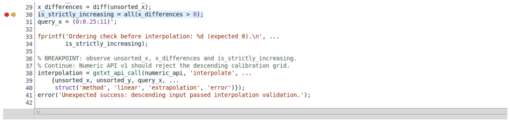
The debugger allows us to inspect variables during execution: the concentration vector is descending and the differences are negative. The strictly increasing condition cannot be satisfied.

After pressing Continue, the script reaches the numerical API call. The service reports the exact problem:
X must be strictly increasing; data are never silently sorted
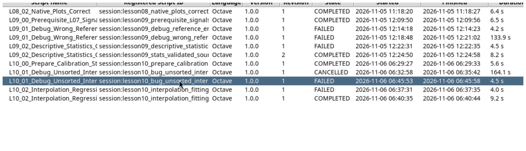
Execution ends with the status FAILED. This is not a malfunction: we deliberately created an invalid script to learn how to recognize a violated precondition. The ordinary Script Runner also records the expected failure with exit code 1.
9. Correcting the error and fitting the models
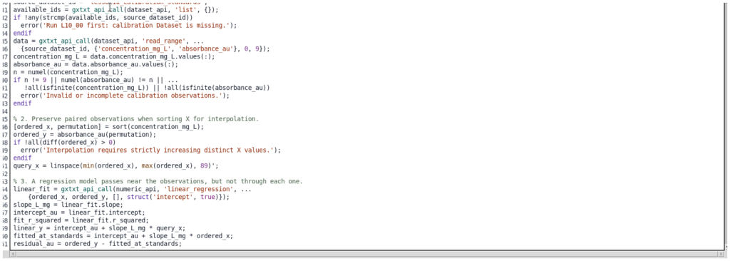
Import L10_02_Interpolation_Regression_Correct.m, assign it a new Script ID and run the Job.
The correction is to sort concentrations together with their corresponding absorbances, rather than removing the validation:
[ordered_x, permutation] = sort(concentration_mg_L);
ordered_y = absorbance_au(permutation);
assert(all(diff(ordered_x) > 0));
9.1 Linear regression
We use the CORE least-squares regression through the public API:
linear_fit = gxtxt_api_call('NUMERIC_API_v1', 'linear_regression', ...
  {ordered_x, ordered_y, [], struct('intercept', true)});
slope_L_mg = linear_fit.slope;
intercept_au = linear_fit.intercept;
fit_r_squared = linear_fit.r_squared;
The arguments are the observation vectors, an optional vector of weights (here [], meaning none was specified) and an options structure requesting the intercept to be fitted. The result contains the line coefficients and its \(R^2\). The regression is unweighted: we are not assuming that different uncertainties are known for the nine standards.
9.2 Piecewise linear interpolation
To construct a curve through the standards, we define a denser grid and call interpolate:
query_x = linspace(min(ordered_x), max(ordered_x), 89)';
interpolated = gxtxt_api_call('NUMERIC_API_v1', 'interpolate', ...
  {ordered_x, ordered_y, query_x, ...
   struct('method', 'linear', 'extrapolation', 'error')});
interpolated_y = interpolated.yq(:);
linspace() generates 89 uniformly spaced X values between the minimum and maximum concentration; the option extrapolation = 'error' prohibits interpolation beyond the available range.
Octave in depth — Evaluating a model with linspace()
linspace(0,11,89) produces 89 X values, including both endpoints, with a constant step of \(11/(89-1)=0.125\) mg/L. These are evaluation points, not new measurements. Increasing the number of plotted points from nine to 89 makes the curves visually smoother, but does not add experimental information or automatically reduce uncertainty.
The trailing apostrophe in linspace(...,89)' transforms the result into a column vector. Domain validation remains essential: generating a denser grid does not authorize calculation beyond the minimum and maximum concentrations of the standards.
9.3 Polynomial fitting
We also calculate a second-degree polynomial:
quadratic_fit = gxtxt_api_call('NUMERIC_API_v1', 'polynomial_fit', ...
  {ordered_x, ordered_y, 2, [], struct('center_scale', true)});
quadratic_y = polyval(quadratic_fit.coefficients(:).', query_x);
The center_scale option improves the numerical stability of fitting. The Octave function polyval() evaluates the polynomial using coefficients returned by the public service; (:).' arranges them as a row vector without conjugation. A higher-order polynomial is useful for comparison, but requires an additional parameter and is not automatically the better model.
Further reading — Quadratic fitting, numerical stability and polyval()
A second-degree polynomial has the form \(\hat A(C)=a_2C^2+a_1C+a_0\), so it has three parameters rather than the line’s two. The option center_scale=true lets the numerical API solve the fitting problem with centered and scaled X values for better conditioning, then return the coefficients in the original concentration basis.
In GNU Octave, polyval([a2,a1,a0],query_x) evaluates the polynomial. The expression coefficients(:).' ensures the coefficients form a row vector, without complex conjugation. Distinguishing coefficient estimation from model evaluation clarifies why polynomial_fit is a GX-TXT numerical-service operation, whereas polyval() is a standard Octave function.
A higher \(R^2\) is not enough to prefer the polynomial: adding parameters also increases the ability to follow random irregularities. Model selection requires physical consistency, inspection of residuals and, when available, independent validation data.
9.4 Numerical results
The analysis gives:
| Quantity | Result |
|---|---|
| Linear intercept \(a\) | 0.01267879 |
| Linear slope \(b\) | 0.08202121 L/mg |
| Linear \(R^2\) | 0.9999628 |
| Residual RMSE | 0.0017482 |
| Quadratic \(R^2\) | 0.9999705 |
| Absorbance of the unknown sample | 0.462 |
| Estimated concentration | 5.478110 mg/L |
The calibration line is:
\[A = 0.01267879 + 0.08202121\, C\]
Inverting the linear model gives the estimated concentration:
\[\hat C_{\mathrm{unknown}} = \frac{A_{\mathrm{unknown}}-a}{b}= 5.478110\ \mathrm{mg/L}\]
The result lies within the 0–11 mg/L standard range. It is therefore an inverse prediction using the calibration model within its domain, not an extrapolation beyond the examined range. This is a teaching example of a point estimate: reporting a real analytical result would also require an uncertainty evaluation.
Analytical chemistry in depth — Inverse prediction and significant figures
To derive concentration from absorbance, solve the line equation for \(C\): \(\hat C=(A-a)/b\). The estimate of 5.478110 mg/L is the numerical result for this synthetic example: six decimal places do not establish experimental accuracy to six decimal places.
In a real experiment, the estimated concentration also depends on the uncertainty of the unknown sample’s absorbance, the scatter of residuals, uncertainty in the standards and the covariance between slope and intercept. Replicate measurements, validated calibration and an uncertainty model would be required. Verifying that the estimate lies between 0 and 11 mg/L avoids extrapolation but does not, by itself, certify analytical quality.
The quadratic model has a slightly higher \(R^2\). That alone is insufficient to select it: an additional parameter can also fit small random fluctuations. Model selection requires residual inspection, model plausibility and, in a laboratory setting, independent standards and validation experiments.
10. Publishing results and viewing plots in GX-TXT
The corrected script publishes four derived Datasets through DATASET_PUBLICATION_API_v2 / publish_series_batch:
lesson10_linear_calibration: response predicted by the straight line.lesson10_piecewise_interpolation: piecewise linearly interpolated curve between standards.lesson10_quadratic_calibration: response predicted by the second-degree polynomial.lesson10_calibration_residuals: difference between observed absorbance and the line’s predicted response.
Each Dataset records Variable IDs, units, the source-data reference and the analysis method. After publication, the program reads back the values with CANONICAL_DATASET_API_v2: this confirms that the stored results match the calculated ones.
For plots, we use PLOT_DATASET_API_v4. The procedure creates a specification with new_spec, fills in its panels, axes and series, validates it with validate_spec, registers it with upsert_plot, renders it with render, and retrieves information using artifacts.
GX-TXT in depth — Persistent plots linked to Datasets
As in Lesson 08, a GX-TXT plot is not an image created independently with figure(). It is a specification registered through PLOT_DATASET_API_v4 that refers to Datasets and their Variable IDs. new_spec prepares the structure, validate_spec checks panels and series, upsert_plot assigns a persistent identity, render creates the visualization, and artifacts returns information about it.
Here one plot compares the standards with three models, while the other shows residuals. They represent numerical results already held in the Session, not independent copies of the data or plotting files written directly to disk.
10.1 Comparing standards, regression line and interpolated curves
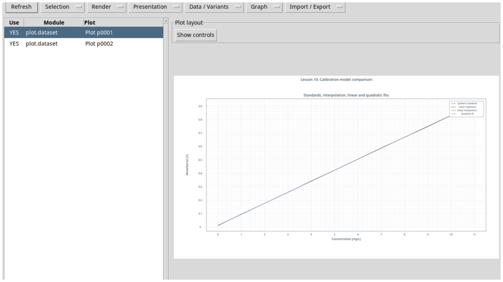
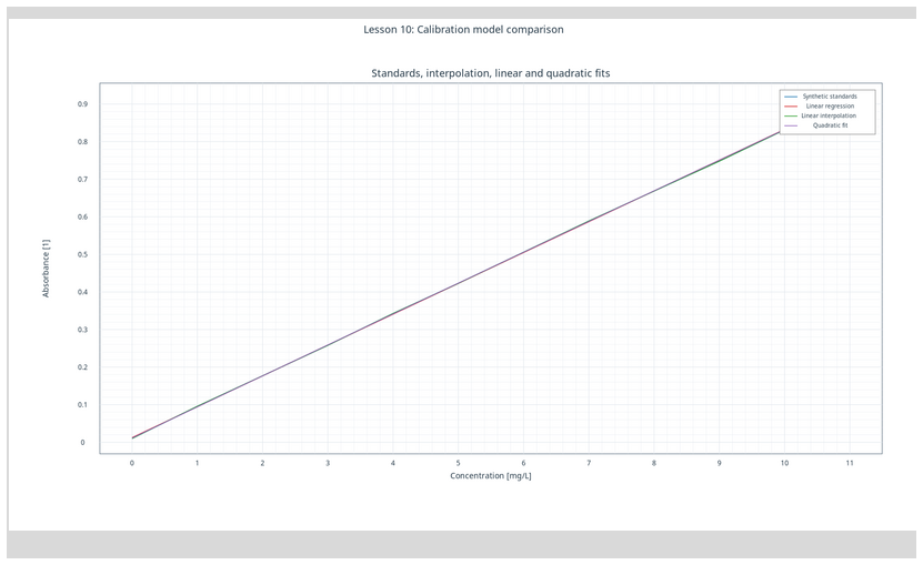
The curves are very close because the chosen relationship is nearly linear. The plot lets us compare their behavior, but visual overlap does not mean the models are mathematically equivalent.
10.2 Residual analysis
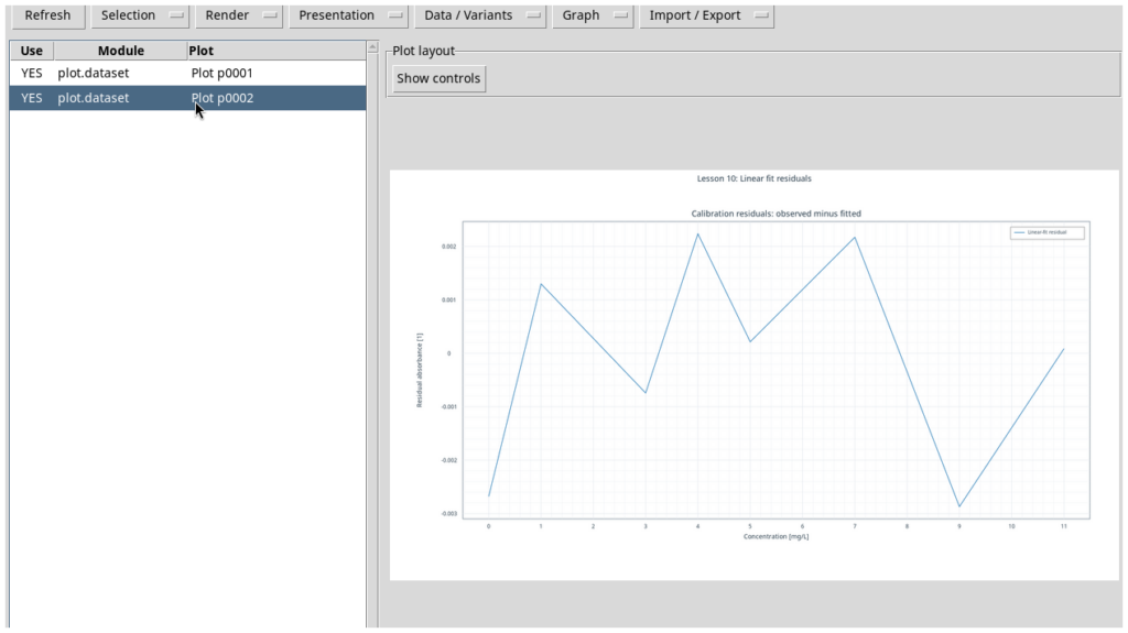
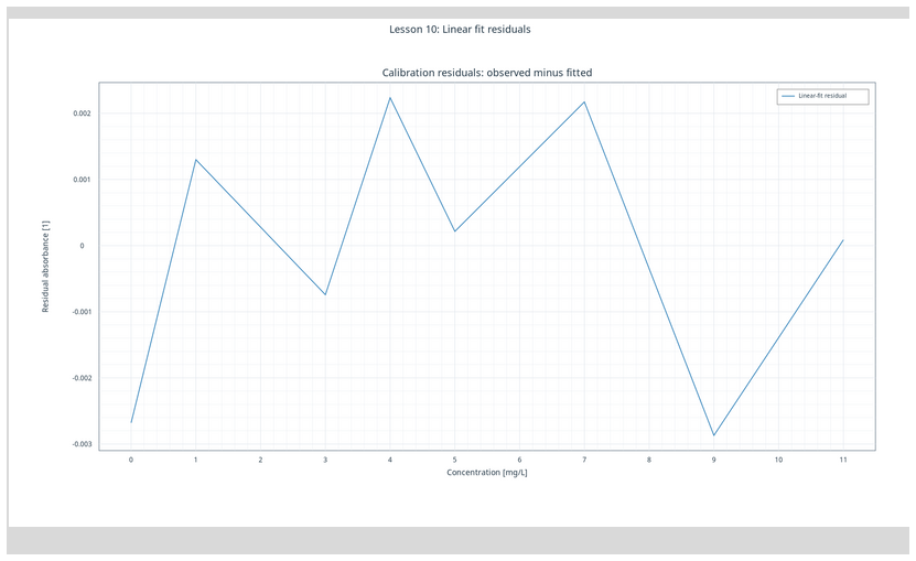
The residuals fluctuate around zero by a few thousandths of an absorbance unit. We need to inspect their pattern, not just the summary \(R^2\) value: systematic curvature, clusters or outliers can reveal model limitations. Nine synthetic standards cannot establish method precision, detection limits or calibration robustness.
Further reading — Scientific interpretation of residuals
An adequate model should leave residuals with no obvious systematic pattern as concentration changes. A curved sequence may suggest a nonlinear relationship; scatter that increases with concentration may indicate heteroscedasticity, meaning nonconstant variance; an isolated point may require checking the corresponding standard.
These clues do not replace statistical testing. Nine synthetic observations let us practice reading a graph, but cannot demonstrate precision, detection limits or freedom from interference for a real analytical method. A residual is a difference in absorbance units, not a concentration.
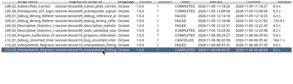
The corrected Job finishes with status COMPLETED and exit code 0. The four Datasets are available in the Session, together with the two persistent plots.
11. Reproducing the experiment and exercises
To reproduce the example: create a new Session, import and run the preparation script first, then debug the intentionally incorrect script and observe the cause of failure. Finally, import and run the corrected script. Check the Datasets and open both plots in the GX-TXT panel.
Suggested exercises:
- Explain why an interpolation grid must be strictly increasing and why sorting only the X values corrupts the experimental pairs.
- Add a synthetic standard at an intermediate concentration; in a fresh Session, recalculate the slope, intercept, \(R^2\) and residuals.
- Introduce an intentionally anomalous data point and examine its effect on the fit and on the estimated unknown concentration.
- Compare the line with the second-degree polynomial: why is the model with the higher \(R^2\) not necessarily preferable?
- Suggest the additional measurements and statistical method needed to assign a credible uncertainty to the unknown concentration.
12. Framework version, sources and license
This lesson uses the public GX-TXT sources from branch maintenance/dev112, commit 125afdb62110a92199f59a066199bb7f2dc7ed68, checked on November 6, 2026. The execution described here used GX-TXT DEV112 Release 2 with patches P001–P005 and the Octave Script Bridge available in that version. Operations and signatures may differ in earlier or later versions.
Technical documentation of the APIs used is available in the repository at the same commit:
- Numeric API v1: interpolation and regression
- Canonical Dataset API v2
- Dataset Publication API v2
- Plot Dataset API v4
- Octave Script Bridge API v1
The three GNU Octave scripts in this lesson are distributed under the GNU GPL v3 or later license. Their complete source code is included in the expandable sections at the end of the article.
13. Complete GNU Octave scripts
The three scripts are reproduced in full below. Expand the corresponding section and copy the code into a .m file, keeping all original English comments.
Script 00 — Preparing synthetic standards (L10_00_Prepare_Calibration_Standards.m)
% Lesson 10 - Prepare a reproducible analytical calibration Dataset.
% Course: GNU Octave with GX-TXT | DEV112 Release 2 + P001-P005
% GitHub commit: 125afdb62110a92199f59a066199bb7f2dc7ed68
% SPDX-License-Identifier: GPL-3.0-or-later
%
% Execute in a NEW GX-TXT Session using the managed Octave Script Workspace.
% This example represents synthetic analytical standards, not real measurements.
% The Dataset is create-only. Do not repeat this script in the same Session.

dataset_api = 'CANONICAL_DATASET_API_v2';
publication_api = 'DATASET_PUBLICATION_API_v2';
gxtxt_api_require({dataset_api, publication_api});
assert(gxtxt_api_has_operation(dataset_api, 'list'));
assert(gxtxt_api_has_operation(dataset_api, 'read_range'));
assert(gxtxt_api_has_operation(publication_api, 'publish_series_batch'));

% Each concentration and absorbance value belongs to one calibration standard.
concentration_mg_L = [0; 1; 2; 3; 4; 5; 7; 9; 11];
absorbance_au = [0.010; 0.096; 0.177; 0.258; 0.343; ...
                 0.423; 0.589; 0.748; 0.915];
n = numel(concentration_mg_L);
assert(n == numel(absorbance_au));
assert(all(isfinite(concentration_mg_L)) && all(isfinite(absorbance_au)));
assert(all(diff(concentration_mg_L) > 0));

source_dataset_id = 'lesson10_calibration_standards';
existing_ids = gxtxt_api_call(dataset_api, 'list', {});
if any(strcmp(existing_ids, source_dataset_id))
  error('Calibration Dataset already exists. Create a fresh Session.');
endif

% A stable Variable ID is not the same thing as a display label.
x_variable = struct('variable_id', 'concentration_mg_L', ...
   'name', 'concentration_mg_L', ...
   'display_label', 'Concentration (synthetic standard)', ...
   'unit', 'mg/L', 'dtype', 'float64', 'value_kind', 'number', ...
   'semantic_source', 'generator');
y_variable = struct('variable_id', 'absorbance_au', ...
   'name', 'absorbance_au', ...
   'display_label', 'Absorbance (synthetic)', ...
   'unit', '1', 'dtype', 'float64', 'value_kind', 'number', ...
   'semantic_source', 'generator');

metadata = struct();
metadata.('simulation.model') = 'synthetic_analytical_calibration';
metadata.('simulation.is_real_measurement') = false;
metadata.('simulation.n_standards') = n;
metadata.('simulation.units_x') = 'mg/L';
metadata.('simulation.units_y') = '1';

request = struct( ...
   'dataset_id', source_dataset_id, 'contract', 'table.generic', ...
   'storage', 'auto', 'x_values', concentration_mg_L, ...
   'y_values', absorbance_au, 'x_variable', x_variable, ...
   'y_variable', y_variable, 'producer_version', '1.0.0', ...
   'source', 'GX-TXT GNU Octave Lesson 10', ...
   'provenance', 'Deterministic synthetic standard concentrations and absorbances', ...
   'notes', 'Artificial data for interpolation and regression education', ...
   'structured_metadata', metadata);
batch_request = struct('series', {{request}});
receipt = gxtxt_api_call(publication_api, 'publish_series_batch', {batch_request});
if !receipt.atomic || receipt.output_count != 1
  error('The public Dataset batch publication was not confirmed.');
endif

% Read back through the public canonical Dataset service, not private files.
readback = gxtxt_api_call(dataset_api, 'read_range', ...
   {source_dataset_id, {'concentration_mg_L', 'absorbance_au'}, 0, n});
assert(max(abs(readback.concentration_mg_L.values(:) - concentration_mg_L)) < 1e-12);
assert(max(abs(readback.absorbance_au.values(:) - absorbance_au)) < 1e-12);
fprintf('PASS: published %d synthetic calibration standards in %s.\n', ...
         n, source_dataset_id);
Script 01 — Intentional error and debugger (L10_01_Debug_Unsorted_Interpolation.m)
% Lesson 10 - Intentional error: unsorted X values in interpolation.
% Course: GNU Octave with GX-TXT | DEV112-P005
% GitHub commit: 125afdb62110a92199f59a066199bb7f2dc7ed68
% SPDX-License-Identifier: GPL-3.0-or-later
%
% Run this script in GX-TXT's native Octave debugger. It MUST fail.
% Place a breakpoint on the interpolate call below. Inspect the X vector,
% the first differences, and the boolean ordering check before continuing.

dataset_api = 'CANONICAL_DATASET_API_v2';
numeric_api = 'NUMERIC_API_v1';
gxtxt_api_require({dataset_api, numeric_api});
assert(gxtxt_api_has_operation(dataset_api, 'read_range'));
assert(gxtxt_api_has_operation(numeric_api, 'interpolate'));

samples = gxtxt_api_call(dataset_api, 'read_range', ...
   {'lesson10_calibration_standards', ...
    {'concentration_mg_L', 'absorbance_au'}, 0, 9});
concentration_mg_L = samples.concentration_mg_L.values(:);
absorbance_au = samples.absorbance_au.values(:);
if numel(concentration_mg_L) != 9 || numel(absorbance_au) != 9
  error('The calibration prerequisites are incomplete.');
endif

% INTENTIONAL BUG: reverse the paired standard observations before interpolating.
% Regression would accept unordered X, but interpolation requires increasing X.
unsorted_x = flipud(concentration_mg_L);
unsorted_y = flipud(absorbance_au);
x_differences = diff(unsorted_x);
is_strictly_increasing = all(x_differences > 0);
query_x = (0:0.25:11)';

fprintf('Ordering check before interpolation: %d (expected 0).\n', ...
        is_strictly_increasing);

% BREAKPOINT: observe unsorted_x, x_differences and is_strictly_increasing.
% Continue: Numeric API v1 should reject the descending calibration grid.
interpolation = gxtxt_api_call(numeric_api, 'interpolate', ...
    {unsorted_x, unsorted_y, query_x, ...
     struct('method', 'linear', 'extrapolation', 'error')});
error('Unexpected success: descending input passed interpolation validation.');
Script 02 — Interpolation, fitting, Datasets and plots (L10_02_Interpolation_Regression_Correct.m)
% Lesson 10 - Fit and interpolate a synthetic analytical calibration.
% Course: GNU Octave with GX-TXT | DEV112 Release 2 + P001-P005
% GitHub commit: 125afdb62110a92199f59a066199bb7f2dc7ed68
% SPDX-License-Identifier: GPL-3.0-or-later
%
% Run after L10_00 in the same fresh Session; outputs are create-only.
% Every scientific Dataset and plot is managed by GX-TXT's public APIs.
% Native GNU Octave syntax is used for vector checks and scalar arithmetic.

dataset_api = 'CANONICAL_DATASET_API_v2';
numeric_api = 'NUMERIC_API_v1';
publication_api = 'DATASET_PUBLICATION_API_v2';
plot_api = 'PLOT_DATASET_API_v4';
gxtxt_api_require({dataset_api, numeric_api, publication_api, plot_api});
required = {
  dataset_api, 'list'; dataset_api, 'read_range';
  numeric_api, 'interpolate'; numeric_api, 'linear_regression';
  numeric_api, 'polynomial_fit';
  publication_api, 'publish_series_batch';
  plot_api, 'new_spec'; plot_api, 'validate_spec';
  plot_api, 'upsert_plot'; plot_api, 'render'; plot_api, 'artifacts'
};
for k = 1:rows(required)
  if !gxtxt_api_has_operation(required{k,1}, required{k,2})
    error('Missing public operation: %s/%s', required{k,1}, required{k,2});
  endif
endfor

% 1. Read the actual published calibration Dataset through stable Variable IDs.
source_dataset_id = 'lesson10_calibration_standards';
available_ids = gxtxt_api_call(dataset_api, 'list', {});
if !any(strcmp(available_ids, source_dataset_id))
  error('Run L10_00 first: calibration Dataset is missing.');
endif
data = gxtxt_api_call(dataset_api, 'read_range', ...
  {source_dataset_id, {'concentration_mg_L', 'absorbance_au'}, 0, 9});
concentration_mg_L = data.concentration_mg_L.values(:);
absorbance_au = data.absorbance_au.values(:);
n = numel(concentration_mg_L);
if n != 9 || numel(absorbance_au) != n || ...
   !all(isfinite(concentration_mg_L)) || !all(isfinite(absorbance_au))
  error('Invalid or incomplete calibration observations.');
endif

% 2. Preserve paired observations when sorting X for interpolation.
[ordered_x, permutation] = sort(concentration_mg_L);
ordered_y = absorbance_au(permutation);
if !all(diff(ordered_x) > 0)
  error('Interpolation requires strictly increasing distinct X values.');
endif
query_x = linspace(min(ordered_x), max(ordered_x), 89)';

% 3. A regression model passes near the observations, but not through each one.
linear_fit = gxtxt_api_call(numeric_api, 'linear_regression', ...
    {ordered_x, ordered_y, [], struct('intercept', true)});
slope_L_mg = linear_fit.slope;
intercept_au = linear_fit.intercept;
fit_r_squared = linear_fit.r_squared;
linear_y = intercept_au + slope_L_mg * query_x;
fitted_at_standards = intercept_au + slope_L_mg * ordered_x;
residual_au = ordered_y - fitted_at_standards;
rmse_au = sqrt(mean(residual_au .^ 2));
if !(isfinite(slope_L_mg) && slope_L_mg > 0 && ...
     isfinite(intercept_au) && isfinite(fit_r_squared))
  error('Regression returned implausible calibration coefficients.');
endif

% 4. Polynomial fitting: a higher R-squared alone cannot select a model.
quadratic_fit = gxtxt_api_call(numeric_api, 'polynomial_fit', ...
    {ordered_x, ordered_y, 2, [], struct('center_scale', true)});
% The polynomial_evaluate API is not available through this Script Bridge.
% Evaluating the public fitted coefficients with native Octave polyval is safe.
% The small physical concentration range avoids severe power-basis conditioning.
quadratic_y = polyval(quadratic_fit.coefficients(:).', query_x);

% 5. Piecewise linear interpolation passes through each standard point.
interpolated = gxtxt_api_call(numeric_api, 'interpolate', ...
    {ordered_x, ordered_y, query_x, ...
     struct('method', 'linear', 'extrapolation', 'error')});
interpolated_y = interpolated.yq(:);
assert(numel(interpolated_y) == numel(query_x));
assert(numel(quadratic_y) == numel(query_x));
assert(all(isfinite(interpolated_y)) && all(isfinite(quadratic_y)));

% 6. Inverse prediction uses the linear calibration model, not interpolation.
unknown_absorbance_au = 0.462;
unknown_concentration_mg_L = ...
    (unknown_absorbance_au - intercept_au) / slope_L_mg;
if unknown_concentration_mg_L < min(ordered_x) || ...
   unknown_concentration_mg_L > max(ordered_x)
  error('Unknown concentration lies outside the calibrated range.');
endif
fprintf('Linear calibration: A = %.8f + %.8f * C [mg/L]\n', ...
       intercept_au, slope_L_mg);
fprintf('Linear R-squared = %.7f; residual RMSE = %.7f AU\n', ...
       fit_r_squared, rmse_au);
fprintf('Quadratic R-squared = %.7f (not automatically better)\n', ...
       quadratic_fit.r_squared);
fprintf('Unknown absorbance %.3f gives concentration %.6f mg/L\n', ...
       unknown_absorbance_au, unknown_concentration_mg_L);

% 7. Publish four independent derived canonical Datasets atomically.
derived_ids = {'lesson10_linear_calibration', ...
               'lesson10_piecewise_interpolation', ...
               'lesson10_quadratic_calibration', ...
               'lesson10_calibration_residuals'};
for k = 1:numel(derived_ids)
  if any(strcmp(available_ids, derived_ids{k}))
    error('Derived Dataset already exists: %s. Use a new Session.', ...
          derived_ids{k});
  endif
endfor

x_variable = struct('variable_id', 'concentration_mg_L', ...
  'name', 'concentration_mg_L', 'display_label', 'Concentration', ...
  'unit', 'mg/L', 'dtype', 'float64', 'value_kind', 'number', ...
  'semantic_source', 'plugin');
absorbance_variable = struct('variable_id', 'absorbance_au', ...
  'name', 'absorbance_au', 'display_label', 'Model absorbance', ...
  'unit', '1', 'dtype', 'float64', 'value_kind', 'number', ...
  'semantic_source', 'plugin');
residual_variable = struct('variable_id', 'residual_au', ...
  'name', 'residual_au', 'display_label', 'Observed minus fitted absorbance', ...
  'unit', '1', 'dtype', 'float64', 'value_kind', 'number', ...
  'semantic_source', 'plugin');
x_values = {query_x, query_x, query_x, ordered_x};
y_values = {linear_y, interpolated_y, quadratic_y, residual_au};
y_variables = {absorbance_variable, absorbance_variable, ...
               absorbance_variable, residual_variable};
methods = {'linear least squares', 'piecewise linear interpolation', ...
           'degree-two polynomial least squares', 'linear fit residuals'};
series = cell(1, numel(derived_ids));
for k = 1:numel(derived_ids)
  meta = struct();
  meta.('analysis.method') = methods{k};
  meta.('analysis.input_dataset_id') = source_dataset_id;
  meta.('analysis.linear_r_squared') = fit_r_squared;
  meta.('analysis.unknown_concentration_mg_L') = unknown_concentration_mg_L;
  series{k} = struct('dataset_id', derived_ids{k}, ...
    'contract', 'table.generic', 'storage', 'auto', ...
    'x_values', x_values{k}, 'y_values', y_values{k}, ...
    'x_variable', x_variable, 'y_variable', y_variables{k}, ...
    'producer_version', '1.0.0', 'source', 'GX-TXT Octave Lesson 10', ...
    'provenance', 'Derived from synthetic calibration standards via public APIs', ...
    'source_dataset_ids', {{source_dataset_id}}, ...
    'notes', methods{k}, 'structured_metadata', meta);
endfor
request = struct('series', {series});
receipt = gxtxt_api_call(publication_api, 'publish_series_batch', {request});
if !receipt.atomic || receipt.output_count != numel(derived_ids)
  error('Atomic batch publication did not confirm four derived Datasets.');
endif

% 8. Verify persistent scientific values via the public Dataset reader.
all_ids = gxtxt_api_call(dataset_api, 'list', {});
for k = 1:numel(derived_ids)
  if !any(strcmp(all_ids, derived_ids{k}))
    error('Published Dataset missing: %s.', derived_ids{k});
  endif
  saved = gxtxt_api_call(dataset_api, 'read_range', ...
      {derived_ids{k}, {'concentration_mg_L', ...
      y_variables{k}.variable_id}, 0, numel(y_values{k})});
  recovered = saved.(y_variables{k}.variable_id).values(:);
  if numel(recovered) != numel(y_values{k}) || ...
     max(abs(recovered - y_values{k})) > 1e-9
    error('Public read-back failed for: %s.', derived_ids{k});
  endif
endfor

% 9. Create persistent native GX-TXT plots using canonical Dataset references.
comparison = gxtxt_api_call(plot_api, 'new_spec', ...
    {'plot.dataset.xy', 'Lesson 10: Calibration model comparison'});
p = comparison.panels{1};
p.id = 'calibration_comparison';
p.title = 'Standards, interpolation, linear and quadratic fits';
p.axes = struct('x', ...
    struct('label', 'Concentration [mg/L]', 'scale', 'linear'), ...
    'y_left', struct('label', 'Absorbance [1]', 'scale', 'linear'));
p.series = {
  struct('id', 'standards', 'label', 'Synthetic standards', ...
      'dataset_id', source_dataset_id, ...
      'x_variable_id', 'concentration_mg_L', ...
      'y_variable_id', 'absorbance_au', 'axis', 'left', 'kind', 'line'),
  struct('id', 'linear', 'label', 'Linear regression', ...
      'dataset_id', derived_ids{1}, ...
      'x_variable_id', 'concentration_mg_L', ...
      'y_variable_id', 'absorbance_au', 'axis', 'left', 'kind', 'line'),
  struct('id', 'piecewise', 'label', 'Linear interpolation', ...
      'dataset_id', derived_ids{2}, ...
      'x_variable_id', 'concentration_mg_L', ...
      'y_variable_id', 'absorbance_au', 'axis', 'left', 'kind', 'line'),
  struct('id', 'quadratic', 'label', 'Quadratic fit', ...
      'dataset_id', derived_ids{3}, ...
      'x_variable_id', 'concentration_mg_L', ...
      'y_variable_id', 'absorbance_au', 'axis', 'left', 'kind', 'line')
};
comparison.panels = {p};
if !gxtxt_api_call(plot_api, 'validate_spec', {comparison})
  error('The model comparison PlotSpec is invalid.');
endif
plot_ref = gxtxt_api_call(plot_api, 'upsert_plot', ...
    {'lesson10_calibration_comparison', comparison});
gxtxt_api_call(plot_api, 'render', {plot_ref});
comparison_artifacts = gxtxt_api_call(plot_api, 'artifacts', {plot_ref});

residual_spec = gxtxt_api_call(plot_api, 'new_spec', ...
    {'plot.dataset.xy', 'Lesson 10: Linear fit residuals'});
r = residual_spec.panels{1};
r.id = 'residuals';
r.title = 'Calibration residuals: observed minus fitted';
r.axes = struct('x', ...
    struct('label', 'Concentration [mg/L]', 'scale', 'linear'), ...
    'y_left', struct('label', 'Residual absorbance [1]', 'scale', 'linear'));
r.series = {struct('id', 'residual', 'label', 'Linear-fit residual', ...
    'dataset_id', derived_ids{4}, 'x_variable_id', 'concentration_mg_L', ...
    'y_variable_id', 'residual_au', 'axis', 'left', 'kind', 'line')};
residual_spec.panels = {r};
if !gxtxt_api_call(plot_api, 'validate_spec', {residual_spec})
  error('The residual PlotSpec is invalid.');
endif
residual_ref = gxtxt_api_call(plot_api, 'upsert_plot', ...
    {'lesson10_calibration_residuals', residual_spec});
gxtxt_api_call(plot_api, 'render', {residual_ref});
residual_artifacts = gxtxt_api_call(plot_api, 'artifacts', {residual_ref});

fprintf('PASS: 4 canonical Datasets, 2 native plots, read-back verified.\n');
disp(comparison_artifacts);
disp(residual_artifacts);
Other steps of this project
- Lesson 01 — Your First GNU Octave Script in GX-TXT
- Lesson 02 — Variables, Data Types and Operators in GNU Octave with GX-TXT
- Lesson 03 — Vectors and Matrices in GNU Octave with GX-TXT: Temperature Measurement Analysis
- Lesson 04 — Conditions, Loops, and Functions. Simulating Newton’s Law of Cooling
- Lesson 05: Scientific Datasets and Variable IDs
- Lesson 06 — Selecting and Reading Experimental Data with GNU Octave and GX-TXT