

Lesson 12 – Linear Algebra: Analyzing a Spectrophotometric Mixture with GNU Octave and GX-TXT
A system of linear equations makes it possible to determine unknown concentrations from several measurements at once. In this lesson, we prepare a synthetic three-component spectrophotometric mixture, recover its concentrations, investigate the loss of matrix rank, and learn how to interpret singular values. We will use GNU Octave within GX-TXT and only the framework’s public APIs.
Reference version: GX-TXT 0.9.8.10-dev-112 Release 2 P008, GitHub release, verified commit 17ff2a7f93de0612015a873e626f87dbeb56b6a2. API contract version numbers are distinct from the GX-TXT distribution version.
Learning objectives
We will learn to construct matrices and vectors; use rows, columns, and size; distinguish matrix multiplication from element-wise multiplication; recognize matrix rank and conditioning; solve overdetermined systems by least squares; interpret the SVD; and publish persistent Datasets and plots in GX-TXT. This lesson builds on the statistical and numerical methods introduced in Lessons 09, 10, and 11.
Continuity with Lessons 01–11
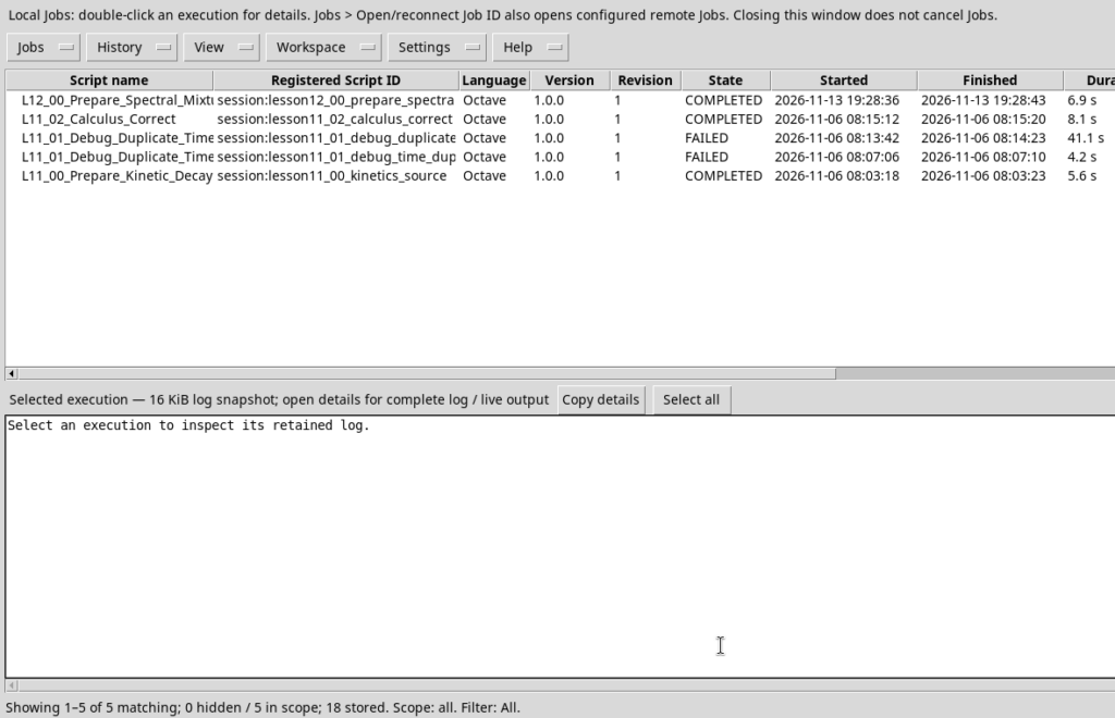
This exercise introduces new mathematical methods but reuses familiar tools: Lessons 01–04 (Script Bridge, numeric types, matrices, functions, conditions, and loops), 05–06 (Datasets, Variable IDs, and canonical reading), 07 (atomic publication), 08 (Plot Dataset and debugger), 09 (statistics and residuals), 10 (interpolation, regression, and fitting), and 11 (numerical differentiation and integration).
| Previously covered | New in Lesson 12 |
|---|---|
| Matrices and matrix multiplication (03) | Rank, rectangular systems, and the geometric meaning of columns |
| Fitting and residuals (10) | Simultaneous estimation of three concentrations from five observations |
| Data statistics (09) | Distinguishing residual goodness of fit from model identifiability |
| Debugger and checks (08–11) | Scientific error due to rank deficiency and SVD diagnosis |
| GX-TXT numerical APIs | linear_matrix: inspect, solve, multiply, and svd |
The word rank needs clarification: in Lesson 05, the rank field of a variable descriptor indicated the number of dimensions of an array (for example, 1 for a vector). Here, rank(A) instead denotes the number of linearly independent columns or rows of a matrix. These are different concepts, even though they share the same term.
1. The scientific problem
Three species, A, B, and C, absorb light at different wavelengths. We collect five absorbance values at 420, 460, 500, 540, and 580 nm. The Beer–Lambert law for the mixture is:
\[a_i=\ell\sum_{j=1}^{3}\varepsilon_{ij}c_j+\eta_i\]
The optical path length is \(\ell=1\) cm; \(\varepsilon_{ij}\) is the absorption coefficient of species \(j\), \(c_j\) its concentration, and \(\eta_i\) a small synthetic perturbation. In matrix form:
\[\mathbf b=\mathbf A\mathbf c+\boldsymbol\eta,\qquad \mathbf A=\ell\boldsymbol\varepsilon\]
The matrix \(\mathbf A\) has 5 rows and 3 columns: five absorbance measurements are used to estimate three concentrations. The data are synthetic and deterministic: they are not actual measurements.
| Wavelength (nm) | Coeff. A | Coeff. B | Coeff. C | Absorbance |
|---|---|---|---|---|
| 420 | 0.115 | 0.020 | 0.015 | 0.2235 |
| 460 | 0.092 | 0.056 | 0.018 | 0.2180 |
| 500 | 0.054 | 0.097 | 0.038 | 0.2241 |
| 540 | 0.024 | 0.078 | 0.101 | 0.2419 |
| 580 | 0.010 | 0.030 | 0.133 | 0.2139 |
The coefficient units are L/(mmol·cm), the concentration units are mmol/L, and absorbance is dimensionless.
1.1 Why multiple wavelengths are needed
At a single wavelength, the absorbance of a mixture provides just one equation involving three unknown concentrations: in general, this is insufficient to determine A, B, and C uniquely. Measuring at five wavelengths gives five equations for three unknowns. The three columns of the matrix represent the response of each component at the five wavelengths.
With an optical path length of 1 cm, the absorption-coefficient matrix becomes a matrix A with units of L/mmol. The product A*c, with c expressed in mmol/L, is therefore dimensionless, as absorbance must be. Checking units helps reveal mistakes that a numerical algorithm cannot detect.
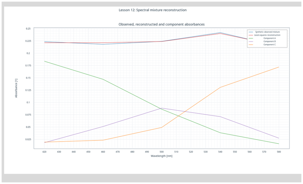
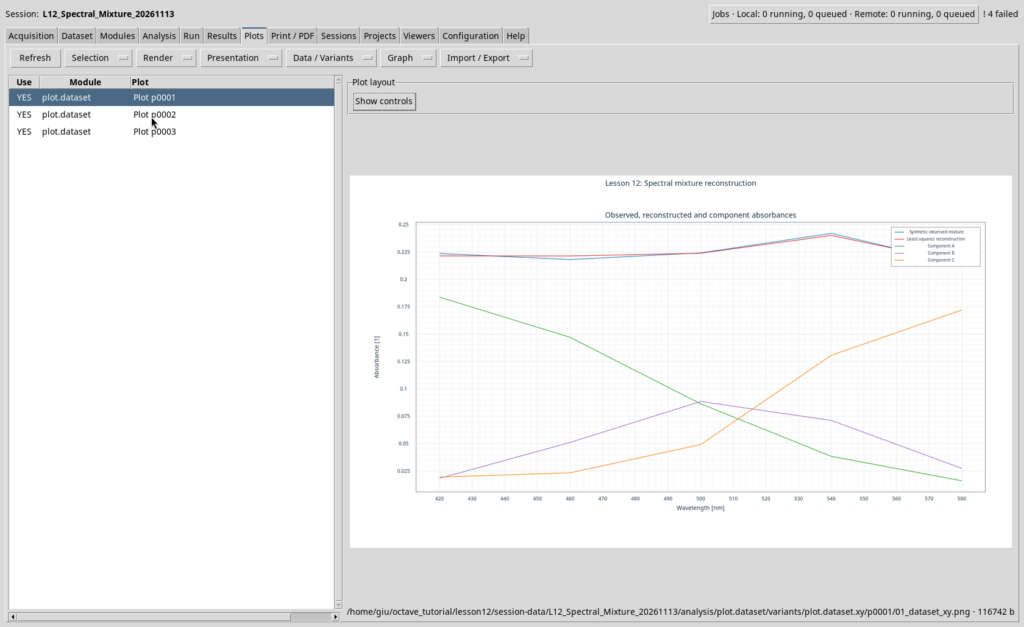
The five points are not a continuous UV–Vis spectrum: they are five discrete synthetic measurements. Lines joining the plotted points are a visual aid, not additional experimental information.
2. Matrices in GNU Octave
Matrix rows are separated by semicolons. Column vectors use the same separator:
A = [0.115, 0.020, 0.015;
     0.092, 0.056, 0.018;
     0.054, 0.097, 0.038;
     0.024, 0.078, 0.101;
     0.010, 0.030, 0.133];
b = [0.2235; 0.2180; 0.2241; 0.2419; 0.2139];

rows(A)
columns(A)
size(A)
The * operator performs matrix multiplication, whereas .* multiplies elements one by one. For the real-valued data in this lesson, ’ gives the transpose; for complex matrices, it also applies complex conjugation, whereas .’ performs only the transpose.
An independent Octave solution can be computed with A \ b. The complete scientific example instead uses NUMERIC_API_v1/linear_matrix so that GX-TXT CORE performs the computation. The Octave solution serves only as a numerical cross-check. We avoid inv(A)*b: the matrix is not square here, and explicitly forming an inverse is often a poor numerical choice more generally.
2.1 Dimensions and compatibility: the rule before calculation
The matrix A is 5×3, the concentration vector c is 3×1, and the absorbance vector b is 5×1. The product A*c is defined because the inner dimensions match (3 and 3), producing a 5×1 vector. By contrast, c*A is not defined in this example.
\[\underbrace{\mathbf A}_{5\times 3}\,\underbrace{\mathbf c}_{3\times 1}=\underbrace{\widehat{\mathbf b}}_{5\times 1}\]
The .* operator instead performs element-wise multiplication and requires dimensions compatible with Octave’s expansion rules. It does not replace matrix multiplication. The transpose must also be chosen carefully: A' conjugates complex elements, while A.' transposes without conjugation.
A = [1, 2; 3, 4; 5, 6];  % 3x2 matrix
c = [2; 1];                 % 2x1 column vector
b = A * c;                 % 3x1 result
assert(isequal(size(b), [3, 1]));
disp(b);
This pure-Octave example isolates the concept of matrix dimensions; the lesson’s main scientific calculation subsequently uses the public NUMERIC_API_v1 service.
3. First script: create and publish four Datasets
Create a new standalone Session, open Viewers → Octave Scripts, import L12_00_Prepare_Spectral_Mixture.m, assign a Script ID, and save. Start the Job through Run → Open Script Runner. Four Datasets will be created: three component absorption-coefficient spectra and the observed mixture spectrum. The data are immediately read back to verify that publication preserved the correct values.
Dataset APIs
CANONICAL_DATASET_API_v2 defines canonical reading: the list operation returns the available identifiers; read_range(dataset_id, variable_ids, start, count) reads the variables identified by their stable Variable IDs, avoiding direct access to internal files or dependence on column order.
DATASET_PUBLICATION_API_v2 handles publication: publish_series_batch accepts a structure with a series field containing specifications with Dataset IDs, X/Y vectors, variable descriptors, units, provenance, and metadata. The result includes a receipt with atomic and output_count fields, which must be checked.
dataset_ids = gxtxt_api_call('CANONICAL_DATASET_API_v2', 'list', {});
data = gxtxt_api_call('CANONICAL_DATASET_API_v2', 'read_range', ...
  {'lesson12_mixture_observed', {'wavelength_nm', 'absorbance_au'}, 0, 5});
observed = data.absorbance_au.values(:);
This syntax also illustrates access to fields of an Octave structure: data.absorbance_au.values.
4. The Script Bridge and the new linear algebra API
OCTAVE_SCRIPT_BRIDGE_API_v1 provides the public connection between a managed Octave script and the APIs registered by GX-TXT. gxtxt_api_require checks prerequisites and capabilities, gxtxt_api_has_operation checks whether a specific operation is available, and gxtxt_api_call performs a call using positional arguments in a cell array. We do not launch the Bridge manually: the GX-TXT Job manages it.
The NUMERIC_API_v1 / linear_matrix operation provides inspect, solve, multiply, svd, and other algebraic actions. In this release, matrices must be wrapped in structures containing equally sized real and imaginary parts to pass correctly through the Script Bridge. For real matrices, the imaginary part is a matrix of zeros.
gxtxt_api_require({'NUMERIC_API_v1@1:math.numeric+complex_linear_algebra'});
A_node = struct('real', A, 'imaginary', zeros(size(A)));
b_node = struct('real', b, 'imaginary', zeros(size(b)));

info = gxtxt_api_call('NUMERIC_API_v1', 'linear_matrix', ...
  {'inspect', A_node, []});
solution = gxtxt_api_call('NUMERIC_API_v1', 'linear_matrix', ...
  {'solve', A_node, b_node});
concentrations = solution.value_real(:);
inspect returns the matrix rank, condition_number, and other properties. solve provides the solution in value_real and value_imaginary, the residuals, residual_norm, relative_residual, and the solution mode. multiply computes a matrix product; svd returns the components of the singular value decomposition.
The complete API contracts are available at a pinned commit: Script Bridge, Numeric API, Canonical Dataset, Dataset Publication, and Plot Dataset v4.
4.1 Why we transport real and imaginary matrices
Octave can represent complex numbers directly, but this version of the public linear_matrix contract requires a structured object with two fields: real and imaginary. Both must have the same shape. For our real matrix, the imaginary part is explicitly provided as zeros(size(A)). This does not simulate complex numbers: it is the documented transport format for the Script Bridge.
4.2 What we ask CORE to do and how to interpret the result
| Public operation | Input | Meaning of the output |
|---|---|---|
| inspect | Matrix A | Numerical rank and conditioning; preliminary assessment of component separability |
| solve | Matrix A and vector b | Least-squares concentrations, residuals, and solution indicators |
| multiply | Matrix A and estimated vector c | Reconstructed absorbance; independent check of the solution |
| svd | Matrix A | U, S, V decomposition and singular values for stability and rank analysis |
Before every call, it is advisable to check that the operation is available using gxtxt_api_has_operation. The mere presence of NUMERIC_API_v1 does not mean that every framework version supports a given operation.
5. Deliberate error: two indistinguishable spectra
Import L12_01_Debug_Rank_Deficient.m with a different Script ID. The script contains the deliberate scientific error:
invalid_matrix = design_matrix;
invalid_matrix(:, 3) = invalid_matrix(:, 2);
Columns 2 and 3 become identical. The matrix rank drops from 3 to 2, so the system can no longer identify B and C separately. Open Run → Debug Session script, set a breakpoint at line 46 of the distributed script, start Start Debug, and examine the variables invalid_matrix, octave_rank, singular_values, inspect.rank, and is_full_column_rank.
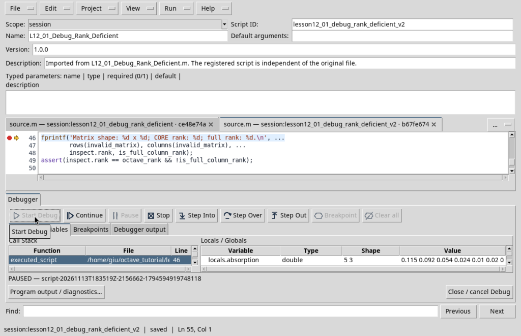
After pressing Continue, CORE rejects the attempt to solve the system with the documented rank-deficiency error. This is the expected outcome: the Job fails to prevent the assignment of physically unidentifiable concentrations.
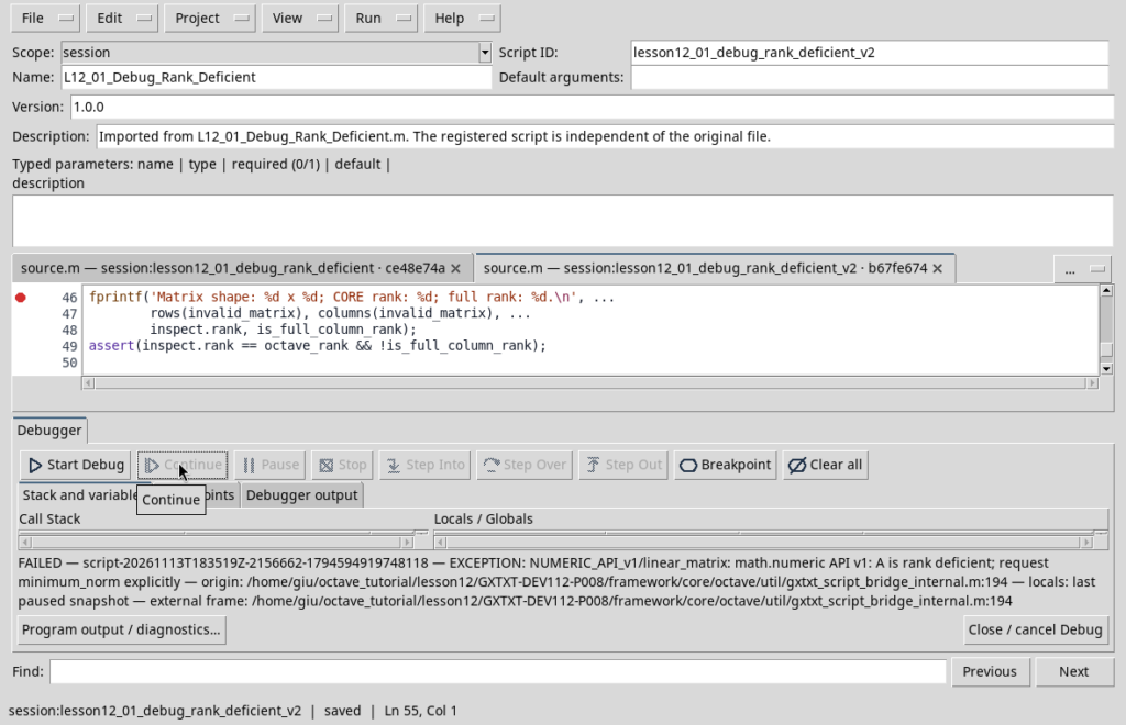
The contract also supports an explicit rank_policy=minimum_norm option for a pseudoinverse-based solution. This does not automatically fix the data: two species with identical spectra remain indistinguishable. We do not use this option in the lesson.
5.1 From rank to chemical identifiability
The maximum rank of a 5×3 matrix is 3. If columns A, B, and C are independent, their contributions can be distinguished mathematically; if two columns coincide, the rank falls to 2. In that case, the concentration of B can be increased and that of C decreased by the same amount without changing the predicted absorbance. The two concentrations cannot be identified separately from the available data.
\[\mathbf A_{B}=\mathbf A_{C}\quad\Longrightarrow\quad \mathbf A\bigl(\mathbf c+t[0,1,-1]^T\bigr)=\mathbf A\mathbf c\]
We need not wait until the columns are exactly equal: if the spectra become nearly identical, the matrix may formally retain rank 3 while becoming ill-conditioned. A small absorbance perturbation can then cause a large change in estimated concentrations. The SVD in Section 7 reveals this transition.
6. Correct solution: least squares
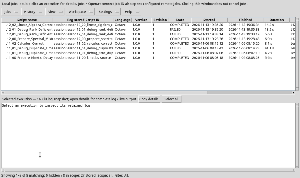
Import L12_02_Linear_Algebra_Correct.m and run it in the same Session. The program rereads the four Datasets, verifies that the wavelength grids match, and constructs a full-column-rank 5×3 matrix. Because the five measurements contain a small amount of noise, we seek the solution that minimizes the sum of squared residuals:
\[\widehat{\mathbf c}=\underset{\mathbf c}{\operatorname{arg\,min}}\;\left\|\mathbf A\mathbf c-\mathbf b\right\|_2^2\]
The public linear_matrix(‘solve’,…) API performs the calculation, while Octave’s A \ b provides an independent cross-check. We avoid explicitly forming the normal equations, which can worsen numerical conditioning.
| Component | Original synthetic concentration | Reconstructed concentration |
|---|---|---|
| A | 1.600000 mmol/L | 1.597382 mmol/L |
| B | 0.900000 mmol/L | 0.911384 mmol/L |
| C | 1.300000 mmol/L | 1.292708 mmol/L |
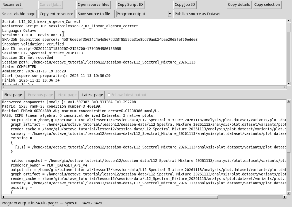
The matrix has rank 3 and a condition number of 3.460109. The RMS residual is 0.00204889 absorbance units; the maximum deviation from the synthetic reference concentrations is 0.01138386 mmol/L. The difference from the original concentrations is due to the synthetic noise introduced before the calculation.
6.1 Why we use least squares rather than an exact solution
In Lesson 10, we estimated the parameters of a calibration curve. Here the fitting principle is similar, but the parameter vector contains three concentrations estimated simultaneously. With five observations and nonzero synthetic noise, there is generally no concentration vector that satisfies every equation exactly. We seek the vector that minimizes the sum of squares of the five deviations.
\[J(\mathbf c)=\sum_{i=1}^{5}\left(b_i-\sum_{j=1}^{3}A_{ij}c_j\right)^2\]
For a matrix with full column rank, the minimum satisfies A'*(A*c-b)=0: the residual vector is orthogonal to the columns of A. This is a mathematical property, not proof that the physical model is correct. In practice, factorizations such as QR or SVD are used for numerical stability, avoiding an explicitly computed inverse or normal equations involving A'*A.
6.2 Interpreting the numerical results
Component B has the greatest deviation from its initial synthetic concentration, with an absolute error of approximately 0.01138 mmol/L. The RMS residual of 0.00204889 is expressed in absorbance units and describes the root-mean-square deviation between the five observations and the reconstructed model. It is not automatically the uncertainty of the concentrations: estimating that would require an explicit statistical model for the noise, its correlations, and the calibration assumptions.
7. Singular values and numerical sensitivity
The linear_matrix(‘svd’,…) action computes the factorization:
\[\mathbf A=\mathbf U\,\mathbf S\,\mathbf V^{T}\]
The singular values \(\sigma_i\) are the diagonal entries of \(\mathbf S\). The 2-norm condition number of a full-rank matrix is:
\[\kappa_2(\mathbf A)=\frac{\sigma_{\max}}{\sigma_{\min}}\]
If \(\sigma_{\min}\) approaches zero, distinguishing some components becomes difficult: small measurement errors can cause large variations in the estimated concentrations. The program numerically checks the reconstruction U*S*V\’ and compares the ratio of singular values with the condition number computed by CORE.
7.1 The geometric meaning of the SVD
The singular value decomposition separates three aspects of the action of a matrix: input orientations, scaling along independent directions, and output orientations. Matrix V identifies combinations of concentrations; S contains the scaling factors (the singular values); and U describes how those combinations appear in absorbance space. Since the data are real, the formula uses the transpose V'. For complex matrices, the conjugate transpose is required.
For the matrix in this lesson, the three singular values are approximately 0.229178, 0.134846, and 0.066234 L/mmol. None is zero, so the rank is 3. The ratio of the largest to the smallest is approximately 3.460109, indicating relatively moderate conditioning in this example. If the smallest value vanished, all the concentrations could not be distinguished.
singular_values = svd(A);
kappa = max(singular_values) / min(singular_values);
fprintf("Condition number = %.6f\n", kappa);
The example just shown is an educational cross-check using Octave’s native svd() function. In the lesson script, the decomposition used for the published results is requested from CORE through NUMERIC_API_v1 / linear_matrix with the svd action.
8. Mixture reconstruction and residuals
The estimated mixture is \(\widehat{\mathbf b}=\mathbf A\widehat{\mathbf c}\). The public linear_matrix(‘multiply’,…) action computes the product, while Octave calculates the individual contributions of the three components.
To visualize the deviations, we define:
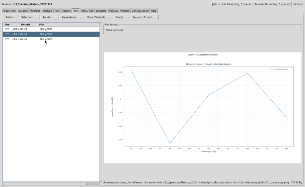
\[r_i=b_i-\widehat b_i\]
Pay attention to the signs: the solve receipt defines the residual as A*c - b, whereas our plot uses b - A*c. The two vectors are negatives of each other; the script explicitly checks this relationship.
8.1 Residuals, sign conventions, and scientific checks
The residual selected for the plot is r = b - A*c_hat, or observed minus reconstructed. Some linear solver APIs instead return A*c_hat - b; the script checks that the two vectors are negatives of each other. The sign reverses the plot vertically but does not change the Euclidean norm or the RMS value.
\[\mathrm{RMS}(\mathbf r)=\sqrt{\frac{1}{5}\sum_{i=1}^{5}r_i^2}\]
A small residual indicates that the model fits these five absorbance values well; it does not, by itself, demonstrate that there are exactly three chemical species, that the coefficients are exact, or that there are no interferences. Analysis of real measurements would require checks of Beer–Lambert linearity, measurement quality, possible spectral overlap, and uncertainty in the spectral coefficients.
9. Six derived Datasets and three native plots
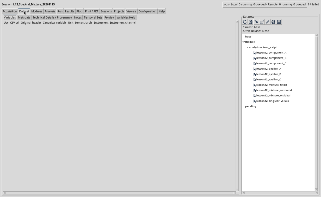
The script publishes the reconstructed mixture, residuals, three component contributions A/B/C, and singular values as Datasets in a single transaction. Every result is read back through the canonical API.
PLOT_DATASET_API_v4 creates persistent scientific plots. new_spec prepares the plot specification, validate_spec checks it, upsert_plot registers a persistent object referencing Dataset IDs and Variable IDs, render generates the representation, and artifacts returns the produced resources. We do not substitute temporary Octave plots for GX-TXT’s scientific plotting system.
9.1 Why derived Datasets remain separate
The observed Dataset remains separate from the reconstructed Dataset because they have different provenance: the former simulates a measurement, while the latter is the result of a mathematical model. The three species contributions, the residual, and the singular values are published as additional canonical Datasets. This extends the atomic publication introduced in Lesson 07 to an inverse analysis.
Plot Dataset v4 objects retain references to Dataset IDs and Variable IDs: they are not merely images exported from Octave. The plots therefore remain linked to the scientific results managed by GX-TXT. Joining the five samples with continuous lines does not mean that intermediate points were acquired.
10. Complete student procedure
- Create a new GX-TXT Session and open Viewers → Octave Scripts.
- Import, register, and run L12_00_Prepare_Spectral_Mixture.m using Run → Open Script Runner.
- Import L12_01_Debug_Rank_Deficient.m with a different Script ID. Open Run → Debug Session script, stop at the breakpoint, and verify rank 2; continue until the expected error occurs.
- Import and run L12_02_Linear_Algebra_Correct.m, using a third Script ID.
- Examine the six derived Datasets and the three plots in the Plots tab.
Datasets have create-only identifiers: use a new Session to repeat the sequence. Do not manually edit CORE registries or files.
Concept checks before moving to the exercises. Students should be able to explain why five equations can estimate three concentrations, what rank 3 means, why rank 2 makes two components indistinguishable, what the condition number measures, why the RMS residual is not the same as concentration uncertainty, and how canonical Datasets make the results reproducible.
11. Exercises
Dimensions. Reduce the number of wavelengths to four and update the matrix and Datasets consistently. What dimensions must the measurement vector have?
Conditioning. Make the spectra of B and C progressively more similar and observe the condition number. What happens to the stability of the concentrations?
Noise. Increase the synthetic noise and compare the RMS residual with the concentration error. Does a smaller residual always guarantee a correct model?
Complex matrices. Construct two small matrices with real and imaginary parts and use linear_matrix(‘multiply’,…); reconstruct the complex result using Octave’s complex function.
Materials
The materials include three GNU Octave scripts with comments exclusively in English, Italian and English guides, real GX-TXT screenshots, and references to the public API contracts. The scripts are distributed under the GNU GPL-3.0-or-later license. This example teaches the distinction between numerical computation alone and building a verifiable, reproducible scientific analysis.
Complete GNU Octave scripts
Expand each section to view and copy the complete source code. All comments are in English.
L12_00_Prepare_Spectral_Mixture.m
% Lesson 12 - Publish a synthetic three-component UV/Vis calibration experiment.
% Course: GNU Octave with GX-TXT | DEV112 Release 2 + P008
% GitHub release: https://github.com/giuxlab-hub/GX-TXT/releases/tag/v0.9.8.10-dev-112-r2-p008
% Pinned public source commit: 17ff2a7f93de0612015a873e626f87dbeb56b6a2
% SPDX-License-Identifier: GPL-3.0-or-later
%
% Run once in a new managed GX-TXT Session.
% All numbers are synthetic educational data, not experimental measurements.
% Extinction coefficients use L/(mmol*cm); optical path length is 1 cm.

dataset_api = 'CANONICAL_DATASET_API_v2';
publication_api = 'DATASET_PUBLICATION_API_v2';
gxtxt_api_require({dataset_api, publication_api});
assert(gxtxt_api_has_operation(dataset_api, 'list'));
assert(gxtxt_api_has_operation(dataset_api, 'read_range'));
assert(gxtxt_api_has_operation(publication_api, 'publish_series_batch'));

wavelength_nm = [420; 460; 500; 540; 580];
epsilon = [0.115, 0.020, 0.015;
           0.092, 0.056, 0.018;
           0.054, 0.097, 0.038;
           0.024, 0.078, 0.101;
           0.010, 0.030, 0.133];
path_length_cm = 1.0;
reference_concentrations_mmol_L = [1.6; 0.9; 1.3];
synthetic_noise_au = [0.002; -0.003; 0.001; 0.002; -0.002];
absorbance_au = (epsilon * path_length_cm) * ...
                reference_concentrations_mmol_L + synthetic_noise_au;
assert(isequal(size(epsilon), [5, 3]));
assert(all(isfinite(epsilon(:))) && all(isfinite(absorbance_au)));
assert(all(diff(wavelength_nm) > 0));

dataset_ids = {'lesson12_epsilon_A', 'lesson12_epsilon_B', ...
               'lesson12_epsilon_C', 'lesson12_mixture_observed'};
available_ids = gxtxt_api_call(dataset_api, 'list', {});
for k = 1:numel(dataset_ids)
  if any(strcmp(available_ids, dataset_ids{k}))
    error('Source Dataset already exists: %s. Use a new Session.', ...
          dataset_ids{k});
  endif
endfor

wavelength_var = struct('variable_id', 'wavelength_nm', ...
  'name', 'wavelength_nm', 'display_label', 'Wavelength', ...
  'unit', 'nm', 'dtype', 'float64', 'value_kind', 'number', ...
  'semantic_source', 'generator');
epsilon_var = struct('variable_id', 'epsilon_L_mmol_cm', ...
  'name', 'epsilon_L_mmol_cm', 'display_label', ...
  'Synthetic molar absorptivity', 'unit', 'L/(mmol*cm)', ...
  'dtype', 'float64', 'value_kind', 'number', ...
  'semantic_source', 'generator');
absorbance_var = struct('variable_id', 'absorbance_au', ...
  'name', 'absorbance_au', 'display_label', 'Synthetic absorbance', ...
  'unit', '1', 'dtype', 'float64', 'value_kind', 'number', ...
  'semantic_source', 'generator');

series = cell(1, 4);
for k = 1:4
  if k <= 3
    values = epsilon(:, k);
    variable = epsilon_var;
    label = sprintf('Synthetic pure-component absorptivity %s', char('A'+k-1));
  else
    values = absorbance_au;
    variable = absorbance_var;
    label = 'Synthetic observed mixture absorbance';
  endif
  metadata = struct();
  metadata.('simulation.synthetic') = true;
  metadata.('simulation.wavelength_count') = numel(wavelength_nm);
  metadata.('simulation.path_length_cm') = path_length_cm;
  metadata.('simulation.model') = 'Beer-Lambert multicomponent linear model';
  metadata.('simulation.series_label') = label;
  series{k} = struct('dataset_id', dataset_ids{k}, ...
    'contract', 'table.generic', 'storage', 'auto', ...
    'x_values', wavelength_nm, 'y_values', values, ...
    'x_variable', wavelength_var, 'y_variable', variable, ...
    'producer_version', '1.0.0', ...
    'source', 'GX-TXT GNU Octave Lesson 12', ...
    'provenance', 'Deterministic synthetic five-wavelength UV/Vis example', ...
    'notes', label, 'structured_metadata', metadata);
endfor
batch = struct('series', {series});
receipt = gxtxt_api_call(publication_api, 'publish_series_batch', {batch});
if !receipt.atomic || receipt.output_count != 4
  error('Atomic publication did not confirm four source Datasets.');
endif

% Read every series back via canonical Dataset and Variable identifiers.
for k = 1:4
  if k <= 3
    y_id = 'epsilon_L_mmol_cm';
    expected = epsilon(:, k);
  else
    y_id = 'absorbance_au';
    expected = absorbance_au;
  endif
  result = gxtxt_api_call(dataset_api, 'read_range', ...
    {dataset_ids{k}, {'wavelength_nm', y_id}, 0, 5});
  assert(max(abs(result.wavelength_nm.values(:) - wavelength_nm)) < 1e-12);
  assert(max(abs(result.(y_id).values(:) - expected)) < 1e-12);
endfor
fprintf('PASS: 4 canonical synthetic source Datasets published and verified.\n');
fprintf('Synthetic reference concentrations [mmol/L]: %.3f %.3f %.3f\n', ...
        reference_concentrations_mmol_L);
L12_01_Debug_Rank_Deficient.m
% Lesson 12 - Intentional rank-deficient linear system for debugging.
% Course: GNU Octave with GX-TXT | DEV112 Release 2 + P008
% GitHub source commit: 17ff2a7f93de0612015a873e626f87dbeb56b6a2
% SPDX-License-Identifier: GPL-3.0-or-later
%
% Run after L12_00 in the same Session. The public solver MUST reject this.
% Set a debugger breakpoint on the marked line before the API call.
% No canonical Dataset or plot is created by this intentionally failing script.

dataset_api = 'CANONICAL_DATASET_API_v2';
numeric_api = 'NUMERIC_API_v1';
gxtxt_api_require({dataset_api, numeric_api});
assert(gxtxt_api_has_operation(dataset_api, 'read_range'));
assert(gxtxt_api_has_operation(numeric_api, 'linear_matrix'));

spectral_ids = {'lesson12_epsilon_A', 'lesson12_epsilon_B', ...
                'lesson12_epsilon_C'};
absorption = zeros(5, 3);
for k = 1:3
  result = gxtxt_api_call(dataset_api, 'read_range', ...
    {spectral_ids{k}, {'wavelength_nm', 'epsilon_L_mmol_cm'}, 0, 5});
  absorption(:, k) = result.epsilon_L_mmol_cm.values(:);
endfor
measurement = gxtxt_api_call(dataset_api, 'read_range', ...
  {'lesson12_mixture_observed', {'wavelength_nm', 'absorbance_au'}, 0, 5});
observed_au = measurement.absorbance_au.values(:);
path_length_cm = 1.0;
design_matrix = absorption * path_length_cm;

% INTENTIONAL SCIENTIFIC ERROR: two components now have identical spectra.
% The matrix columns are linearly dependent; their amounts are not identifiable.
invalid_matrix = design_matrix;
invalid_matrix(:, 3) = invalid_matrix(:, 2);
octave_rank = rank(invalid_matrix);
singular_values = svd(invalid_matrix);
% The Script Bridge transports matrices in explicit real/imaginary envelopes.
invalid_node = struct('real', invalid_matrix, ...
  'imaginary', zeros(size(invalid_matrix)));
observed_node = struct('real', observed_au, ...
  'imaginary', zeros(size(observed_au)));
inspect = gxtxt_api_call(numeric_api, 'linear_matrix', ...
  {'inspect', invalid_node, []});
is_full_column_rank = (inspect.rank == columns(invalid_matrix));

% BREAKPOINT: inspect invalid_matrix, octave_rank, singular_values and inspect.rank.
fprintf('Matrix shape: %d x %d; CORE rank: %d; full rank: %d.\n', ...
        rows(invalid_matrix), columns(invalid_matrix), ...
        inspect.rank, is_full_column_rank);
assert(inspect.rank == octave_rank && !is_full_column_rank);

% No automatic pseudoinverse is requested: the documented default rejects rank loss.
invalid_solution = gxtxt_api_call(numeric_api, 'linear_matrix', ...
  {'solve', invalid_node, observed_node});
error('Unexpected success: rank-deficient system was accepted.');
L12_02_Linear_Algebra_Correct.m
% Lesson 12 - Recover three concentrations with public GX-TXT linear algebra.
% Course: GNU Octave with GX-TXT | DEV112 Release 2 + P008
% GitHub release: https://github.com/giuxlab-hub/GX-TXT/releases/tag/v0.9.8.10-dev-112-r2-p008
% Pinned source commit: 17ff2a7f93de0612015a873e626f87dbeb56b6a2
% SPDX-License-Identifier: GPL-3.0-or-later
%
% Run after L12_00 in a fresh managed GX-TXT Session.
% The calculations use NUMERIC_API_v1/linear_matrix, not a private solver.
% All canonical input/output and plotting operations use public APIs.

dataset_api = 'CANONICAL_DATASET_API_v2';
numeric_api = 'NUMERIC_API_v1';
publication_api = 'DATASET_PUBLICATION_API_v2';
plot_api = 'PLOT_DATASET_API_v4';
gxtxt_api_require({dataset_api, ...
  'NUMERIC_API_v1@1:math.numeric+complex_linear_algebra', ...
  publication_api, plot_api});
required = {
  dataset_api, 'list'; dataset_api, 'read_range';
  numeric_api, 'linear_matrix';
  publication_api, 'publish_series_batch';
  plot_api, 'new_spec'; plot_api, 'validate_spec';
  plot_api, 'upsert_plot'; plot_api, 'render'; plot_api, 'artifacts'
};
for k = 1:rows(required)
  if !gxtxt_api_has_operation(required{k, 1}, required{k, 2})
    error('Missing public operation %s/%s.', required{k, 1}, required{k, 2});
  endif
endfor

% Step 1: read four published source Datasets using stable Variable IDs.
source_ids = {'lesson12_epsilon_A', 'lesson12_epsilon_B', ...
              'lesson12_epsilon_C', 'lesson12_mixture_observed'};
available_ids = gxtxt_api_call(dataset_api, 'list', {});
for k = 1:numel(source_ids)
  if !any(strcmp(available_ids, source_ids{k}))
    error('Missing source Dataset %s: execute L12_00 first.', source_ids{k});
  endif
endfor

n_wavelengths = 5;
wavelength_nm = [];
epsilon = zeros(n_wavelengths, 3);
for k = 1:3
  data = gxtxt_api_call(dataset_api, 'read_range', ...
    {source_ids{k}, {'wavelength_nm', 'epsilon_L_mmol_cm'}, ...
     0, n_wavelengths});
  current_wavelengths = data.wavelength_nm.values(:);
  if k == 1
    wavelength_nm = current_wavelengths;
  elseif max(abs(current_wavelengths - wavelength_nm)) > 1e-12
    error('Component spectra have different wavelength grids.');
  endif
  epsilon(:, k) = data.epsilon_L_mmol_cm.values(:);
endfor
data = gxtxt_api_call(dataset_api, 'read_range', ...
  {source_ids{4}, {'wavelength_nm', 'absorbance_au'}, 0, n_wavelengths});
observed_au = data.absorbance_au.values(:);
if numel(observed_au) != n_wavelengths || ...
   max(abs(data.wavelength_nm.values(:) - wavelength_nm)) > 1e-12 || ...
   !all(isfinite(epsilon(:))) || !all(isfinite(observed_au))
  error('Nonfinite, incomplete, or misaligned spectral observations.');
endif

% Step 2: apply Beer-Lambert units and inspect the overdetermined system.
% epsilon: L/(mmol*cm), path_length: cm, A: L/mmol, c: mmol/L, b: 1.
path_length_cm = 1.0;
A = epsilon * path_length_cm;
b = observed_au;
if !isequal(size(A), [5, 3]) || !isequal(size(b), [5, 1])
  error('Expected a five-row, three-column design matrix and five observations.');
endif
% Explicit matrix envelopes preserve real/imaginary structure across the Bridge.
A_node = struct('real', A, 'imaginary', zeros(size(A)));
b_node = struct('real', b, 'imaginary', zeros(size(b)));
matrix_info = gxtxt_api_call(numeric_api, 'linear_matrix', ...
  {'inspect', A_node, []});
if matrix_info.rank != columns(A) || ...
   !isfinite(matrix_info.condition_number) || ...
   matrix_info.condition_number >= 1e12
  error('Spectral system has insufficient rank or excessive conditioning.');
endif

% Step 3: solve a full-column-rank overdetermined system via the CORE.
% The documented default policy is rank_policy=error, not minimum_norm.
solution = gxtxt_api_call(numeric_api, 'linear_matrix', ...
  {'solve', A_node, b_node});
estimated_mmol_L = solution.value_real(:);
assert(max(abs(solution.value_imaginary(:))) < 1e-12);
assert(numel(estimated_mmol_L) == 3);
assert(all(estimated_mmol_L >= 0) && all(isfinite(estimated_mmol_L)));

% Octave backslash is presented only as a language-learning cross-check.
octave_reference = A \ b;
assert(norm(estimated_mmol_L - octave_reference, Inf) < 1e-9);
assert(solution.rank == 3);
assert(solution.relative_residual < 0.03);

% Step 4: independently reconstruct absorbance using public multiplication.
calculated = gxtxt_api_call(numeric_api, 'linear_matrix', ...
  {'multiply', A_node, ...
   struct('real', estimated_mmol_L, ...
          'imaginary', zeros(size(estimated_mmol_L)))});
fitted_au = calculated.value_real(:);
assert(max(abs(calculated.value_imaginary(:))) < 1e-12);
residual_au = b - fitted_au;
assert(norm(residual_au + solution.residual_real(:)) < 1e-9);
residual_rms_au = sqrt(mean(residual_au .^ 2));
reference_mmol_L = [1.6; 0.9; 1.3];
max_concentration_error_mmol_L = ...
  max(abs(estimated_mmol_L - reference_mmol_L));
if max_concentration_error_mmol_L >= 0.05 || residual_rms_au > 0.004
  error('The synthetic reconstruction failed numerical accuracy checks.');
endif

% Step 5: decompose the coefficient matrix with the public SVD operation.
decomposition = gxtxt_api_call(numeric_api, 'linear_matrix', ...
  {'svd', A_node, []});
U = decomposition.u_real;
S = decomposition.s_real;
V = decomposition.v_real;
assert(norm(U * S * V' - A, 'fro') < 1e-10);
singular_values = diag(S);
assert(numel(singular_values) == 3 && all(singular_values > 0));
assert(abs(max(singular_values) / min(singular_values) - ...
           matrix_info.condition_number) < 1e-8);

% Reconstruct the contribution of each component without inverting A.
component_absorbance_au = A .* repmat(estimated_mmol_L.', n_wavelengths, 1);
assert(max(abs(sum(component_absorbance_au, 2) - fitted_au)) < 1e-10);
fprintf('Recovered components [mmol/L]: A=%.6f B=%.6f C=%.6f.\n', ...
        estimated_mmol_L);
fprintf('Matrix: %dx%d; rank=%d; condition number=%.6f.\n', ...
        rows(A), columns(A), matrix_info.rank, ...
        matrix_info.condition_number);
fprintf('Residual RMS=%.8f AU; maximum concentration error=%.8f mmol/L.\n', ...
        residual_rms_au, max_concentration_error_mmol_L);

% Step 6: publish six derived canonical Datasets in one atomic transaction.
derived_ids = {'lesson12_mixture_fitted', 'lesson12_mixture_residual', ...
  'lesson12_component_A', 'lesson12_component_B', ...
  'lesson12_component_C', 'lesson12_singular_values'};
for k = 1:numel(derived_ids)
  if any(strcmp(available_ids, derived_ids{k}))
    error('Derived Dataset exists: %s. Start a new Session.', derived_ids{k});
  endif
endfor
wavelength_var = struct('variable_id', 'wavelength_nm', ...
  'name', 'wavelength_nm', 'display_label', 'Wavelength', ...
  'unit', 'nm', 'dtype', 'float64', 'value_kind', 'number', ...
  'semantic_source', 'plugin');
index_var = struct('variable_id', 'singular_index', ...
  'name', 'singular_index', 'display_label', 'Singular-value index', ...
  'unit', '1', 'dtype', 'float64', 'value_kind', 'number', ...
  'semantic_source', 'plugin');
absorbance_var = struct('variable_id', 'absorbance_au', ...
  'name', 'absorbance_au', 'display_label', 'Calculated absorbance', ...
  'unit', '1', 'dtype', 'float64', 'value_kind', 'number', ...
  'semantic_source', 'plugin');
residual_var = struct('variable_id', 'residual_au', ...
  'name', 'residual_au', 'display_label', 'Observed minus fitted', ...
  'unit', '1', 'dtype', 'float64', 'value_kind', 'number', ...
  'semantic_source', 'plugin');
singular_var = struct('variable_id', 'singular_value_L_mmol', ...
  'name', 'singular_value_L_mmol', 'display_label', 'Singular value', ...
  'unit', 'L/mmol', 'dtype', 'float64', 'value_kind', 'number', ...
  'semantic_source', 'plugin');

x_values = {wavelength_nm, wavelength_nm, wavelength_nm, ...
            wavelength_nm, wavelength_nm, (1:3)'};
y_values = {fitted_au, residual_au, component_absorbance_au(:, 1), ...
            component_absorbance_au(:, 2), ...
            component_absorbance_au(:, 3), singular_values};
x_variables = {wavelength_var, wavelength_var, wavelength_var, ...
               wavelength_var, wavelength_var, index_var};
y_variables = {absorbance_var, residual_var, absorbance_var, ...
               absorbance_var, absorbance_var, singular_var};
descriptions = {'Least-squares fitted mixture', 'Absorbance residuals', ...
                'Component A absorbance', 'Component B absorbance', ...
                'Component C absorbance', 'Design-matrix singular values'};
series = cell(1, numel(derived_ids));
for k = 1:numel(derived_ids)
  metadata = struct();
  metadata.('analysis.method') = descriptions{k};
  metadata.('analysis.synthetic_source') = true;
  metadata.('analysis.matrix_rank') = matrix_info.rank;
  metadata.('analysis.condition_number') = matrix_info.condition_number;
  metadata.('analysis.residual_rms_au') = residual_rms_au;
  metadata.('analysis.concentration_A_mmol_L') = estimated_mmol_L(1);
  metadata.('analysis.concentration_B_mmol_L') = estimated_mmol_L(2);
  metadata.('analysis.concentration_C_mmol_L') = estimated_mmol_L(3);
  series{k} = struct('dataset_id', derived_ids{k}, ...
    'contract', 'table.generic', 'storage', 'auto', ...
    'x_values', x_values{k}, 'y_values', y_values{k}, ...
    'x_variable', x_variables{k}, 'y_variable', y_variables{k}, ...
    'producer_version', '1.0.0', ...
    'source', 'GX-TXT GNU Octave Lesson 12', ...
    'source_dataset_ids', {source_ids}, ...
    'provenance', 'Synthetic spectral mixture solved through public NUMERIC_API_v1', ...
    'notes', descriptions{k}, 'structured_metadata', metadata);
endfor
receipt = gxtxt_api_call(publication_api, 'publish_series_batch', ...
  {struct('series', {series})});
if !receipt.atomic || receipt.output_count != numel(derived_ids)
  error('Atomic publication did not confirm six derived Datasets.');
endif
for k = 1:numel(derived_ids)
  recovered = gxtxt_api_call(dataset_api, 'read_range', ...
    {derived_ids{k}, ...
     {x_variables{k}.variable_id, y_variables{k}.variable_id}, ...
     0, numel(y_values{k})});
  saved = recovered.(y_variables{k}.variable_id).values(:);
  if numel(saved) != numel(y_values{k}) || ...
     max(abs(saved - y_values{k})) > 1e-9
    error('Public Dataset read-back mismatch: %s.', derived_ids{k});
  endif
endfor

% Step 7: make native GX-TXT Plot Dataset v4 visualizations.
comparison = gxtxt_api_call(plot_api, 'new_spec', ...
  {'plot.dataset.xy', 'Lesson 12: Spectral mixture reconstruction'});
panel = comparison.panels{1};
panel.id = 'spectral_reconstruction';
panel.title = 'Observed, reconstructed and component absorbances';
panel.axes = struct('x', struct('label', 'Wavelength [nm]', 'scale', 'linear'), ...
  'y_left', struct('label', 'Absorbance [1]', 'scale', 'linear'));
panel.series = {
  struct('id', 'measured', 'label', 'Synthetic observed mixture', ...
    'dataset_id', source_ids{4}, 'x_variable_id', 'wavelength_nm', ...
    'y_variable_id', 'absorbance_au', 'axis', 'left', 'kind', 'line'),
  struct('id', 'fitted', 'label', 'Least-squares reconstruction', ...
    'dataset_id', derived_ids{1}, 'x_variable_id', 'wavelength_nm', ...
    'y_variable_id', 'absorbance_au', 'axis', 'left', 'kind', 'line'),
  struct('id', 'A', 'label', 'Component A', ...
    'dataset_id', derived_ids{3}, 'x_variable_id', 'wavelength_nm', ...
    'y_variable_id', 'absorbance_au', 'axis', 'left', 'kind', 'line'),
  struct('id', 'B', 'label', 'Component B', ...
    'dataset_id', derived_ids{4}, 'x_variable_id', 'wavelength_nm', ...
    'y_variable_id', 'absorbance_au', 'axis', 'left', 'kind', 'line'),
  struct('id', 'C', 'label', 'Component C', ...
    'dataset_id', derived_ids{5}, 'x_variable_id', 'wavelength_nm', ...
    'y_variable_id', 'absorbance_au', 'axis', 'left', 'kind', 'line')
};
comparison.panels = {panel};
if !gxtxt_api_call(plot_api, 'validate_spec', {comparison})
  error('Spectral comparison PlotSpec is invalid.');
endif
comparison_ref = gxtxt_api_call(plot_api, 'upsert_plot', ...
  {'lesson12_spectral_reconstruction', comparison});
gxtxt_api_call(plot_api, 'render', {comparison_ref});
comparison_artifacts = gxtxt_api_call(plot_api, 'artifacts', {comparison_ref});

residual_plot = gxtxt_api_call(plot_api, 'new_spec', ...
  {'plot.dataset.xy', 'Lesson 12: Spectral residuals'});
rp = residual_plot.panels{1};
rp.id = 'spectral_residual';
rp.title = 'Observed minus reconstructed absorbance';
rp.axes = struct('x', struct('label', 'Wavelength [nm]', 'scale', 'linear'), ...
  'y_left', struct('label', 'Absorbance residual [1]', 'scale', 'linear'));
rp.series = {struct('id', 'residual', 'label', 'Least-squares residual', ...
  'dataset_id', derived_ids{2}, 'x_variable_id', 'wavelength_nm', ...
  'y_variable_id', 'residual_au', 'axis', 'left', 'kind', 'line')};
residual_plot.panels = {rp};
if !gxtxt_api_call(plot_api, 'validate_spec', {residual_plot})
  error('Residual PlotSpec is invalid.');
endif
residual_ref = gxtxt_api_call(plot_api, 'upsert_plot', ...
  {'lesson12_spectral_residual', residual_plot});
gxtxt_api_call(plot_api, 'render', {residual_ref});
residual_artifacts = gxtxt_api_call(plot_api, 'artifacts', {residual_ref});

sv_plot = gxtxt_api_call(plot_api, 'new_spec', ...
  {'plot.dataset.xy', 'Lesson 12: Spectral matrix singular values'});
sp = sv_plot.panels{1};
sp.id = 'singular_values';
sp.title = 'Singular values of the five-by-three spectral matrix';
sp.axes = struct('x', struct('label', 'Singular-value index', 'scale', 'linear'), ...
  'y_left', struct('label', 'Singular value [L/mmol]', 'scale', 'linear'));
sp.series = {struct('id', 'sv', 'label', 'Singular values', ...
  'dataset_id', derived_ids{6}, 'x_variable_id', 'singular_index', ...
  'y_variable_id', 'singular_value_L_mmol', ...
  'axis', 'left', 'kind', 'line')};
sv_plot.panels = {sp};
if !gxtxt_api_call(plot_api, 'validate_spec', {sv_plot})
  error('Singular-value PlotSpec is invalid.');
endif
sv_ref = gxtxt_api_call(plot_api, 'upsert_plot', ...
  {'lesson12_singular_values', sv_plot});
gxtxt_api_call(plot_api, 'render', {sv_ref});
sv_artifacts = gxtxt_api_call(plot_api, 'artifacts', {sv_ref});

fprintf('PASS: CORE linear algebra, 6 canonical derived Datasets, 3 native plots.\n');
disp(comparison_artifacts);
disp(residual_artifacts);
disp(sv_artifacts);
Other steps of this project
- Lesson 01 — Your First GNU Octave Script in GX-TXT
- Lesson 02 — Variables, Data Types and Operators in GNU Octave with GX-TXT
- Lesson 03 — Vectors and Matrices in GNU Octave with GX-TXT: Temperature Measurement Analysis
- Lesson 04 — Conditions, Loops, and Functions. Simulating Newton’s Law of Cooling
- Lesson 05: Scientific Datasets and Variable IDs
- Lesson 06 — Selecting and Reading Experimental Data with GNU Octave and GX-TXT