

Precision, Aggregation and Basic Statistics
Scientific Python in GX-TXT · Module 3 · Lesson 17
A number of numbers can be summarised, average and dispersion. These numbers are only useful if we know what data has been included, what conventions have been used and what they represent. We will compare NumPy with GX-TXT’s public statistics on the already published synthetic series.
Objectives: to use np.sum, np.mean and np.std; to distinguish population and sample with ddof; to recognize non-finished values and floating point accuracy limits; to compare results with a motivated tolerance.
Prerequisites: Dataset of lesson 9 and array of lessons 13–16.
Summa and media
For the four synthetic [1.2, 1.5, 1.3, 1.6] mV signals, the sum is 5.6 mV and the average is \(\frac{5{.}6}{4}=1{.}4\) mV. Hand control helps to interpret the output of functions:
import numpy as np
signal = np.array([1.2, 1.5, 1.3, 1.6])
print(np.sum(signal))
print(np.mean(signal))
These data are chosen for the exercise, are not experimental measures and have no uncertainty assigned. An average does not describe the dispersion alone or guarantees that the observations are independent.
Standard deviation and ddof
The variance measures the square dispersion around the average; the standard deviation is its square root and has the same unit of data. For the four values of the example, the sum of square waste is 0.1 mV².
With the population convention, we divide for n = 4: the variance is 0.025 mV² and the standard deviation is about 0.1581 mV. With the sample convention, we divide for \(n-1=3\): the variance is about 0.03333 mV² and the standard deviation is about 0.1826 mV.
In NumPy, np.std(signal, ddof=0) uses n, while ddof=1 uses n − 1. Do not choose a convention only because it produces the desired number: the choice depends on demand and assumptions. For n <= ddof, the divider is not positive and the result is not a valid estimate; it controls the sample size.
Missing and unfinished data
An array can contain NaN or infinite. np.mean and np.std can propagate NaN; functions such as np.nanmean adopt a different policy and ignore NaN. Ignoring missing values without declaring it can alter interpretation. It counts the values included and excluded, keeps the information on their origin and chooses the policy according to the problem. A missing cell mask provided by a Dataset should not be automatically identified with each explicit NaN.
The synthetic series of this lesson contains four finite values. The provider’s statistics show four valid values and no unfinished value.
Accuracy and comparison
float64 arrays have finished accuracy. Somme made in different orders can produce small scraps, especially with very different scale values. A comparison between two implementations should use absolute and/or relative tolerance motivated by data scale and purpose; np.isclose(a, b, rtol=..., atol=...) is a possible tool, but its parameters should be consciously chosen. Numerical tolerance is not automatically physical uncertainty.
An analytical control, such as the average of this small hand calculated series, helps to identify a unit error or a different convention. For complex work, it also assesses numerical stability, size and quality of the sample.
Public statistics GX-TXT
We read four lines of signal with CANONICAL_DATASET_API_v2/read_range. Then NUMERIC_API_v1/dataset_statistics receives the Dataset identifier, the variable identifier and an option dictionary. The structured result includes counts, sums, media and statistics of population and samples; the units reported are from the Dataset variable.
The Dataset of lesson 9 must be present at the Session. The bed array is a (4, 1) column in the performance shown: we transform it into a single-dimensional vector with reshape(-1) because we know we have a single column. For multidimensional data it is necessary to check the axes before flattening.
Full code
import numpy as np
from gxtxt import gxtxt_api_call, gxtxt_api_require

gxtxt_api_require("NUMERIC_API_v1@1")
gxtxt_api_require("CANONICAL_DATASET_API_v2@2")
chunk = gxtxt_api_call("CANONICAL_DATASET_API_v2", "read_range", ["corso_python_serie_sintetica", ["segnale"], 0, 4])
signal = np.asarray(chunk["segnale"]["values"]).reshape(-1)
print("Synthetic signal (mV):", signal)
print("Somma (mV):", np.sum(signal))
print("Media (mV):", np.mean(signal))
print("Standard population deviation (mV):", np.std(signal, ddof=0))
print("Standard sample deviation (mV):", np.std(signal, ddof=1))
result = gxtxt_api_call("NUMERIC_API_v1", "dataset_statistics", ["corso_python_serie_sintetica", "segnale", {}])
print("Statistics GX-TXT:", result)
The comparison is valid here because both operations use the same variable and all four rows, without unfinished values. In a general case, check that selection, missing data policy and conventions coincide before comparing the figures.
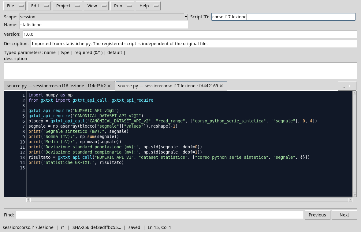
The script compares NumPy aggregations with dataset statistics.
Execution and control
- Open the Session containing
corso_python_serie_sinteticaand the Viewer Python Scripts. - Import
statistics.py, assigns name and Script ID into thesessionbroom, then saves. - Open the Runner, press Run Job and read the output.
- Check
5.6, average1.4, standard population deviation about0.1581and sampling about0.1826mV. In the result GX-TXT comparessum,mean,std_populationandstd_sample.

The output shows NumPy results and GX-TXT statistics descriptor.
Common error
Compare the standard deviation of population of one program with that sample of another and conclude that one of the two is wrong can be misleading. First check the divider, the values included, the units and the treatment of the missing.
Exercise
For synthetic values [2.0, 4.0] mV calculates average and standard population deviation. What is the standard sample deviation?
Worked solution
The average is 3.0 mV. Discards are −1 and 1 mV: the population variance is \(\frac{1+1}{2}=1\,\mathrm{mV}^{2}\), so the standard deviation is 1 mV. The sample variance is \(\frac{1+1}{1}=2\,\mathrm{mV}^{2}\), with standard deviation \(\sqrt{2}\approx1{.}414\,\mathrm{mV}\). These numbers describe the example, not a complete experimental uncertainty.
In the next lesson we will write a managed output file and publish it with the expected APIs.