Build a comparison
Sources, ordering, comparison modes, normalization, and thresholds.
Build the source list
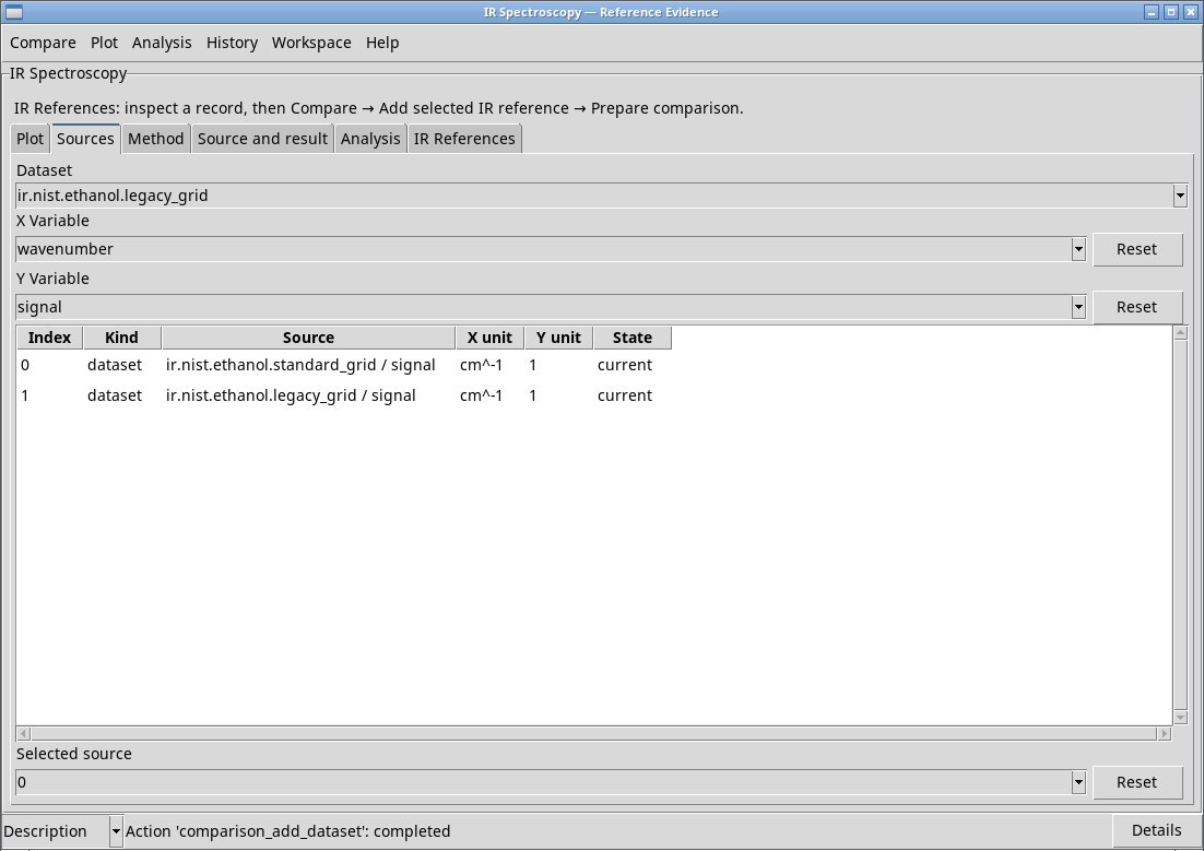
- Open Sources. Use Compare → Discover sources to refresh the eligible Datasets in the session. Select the Dataset. Run discovery again if the variable fields are empty.
- Select X Variable and Y Variable. For the Generators in this guide, choose
wavenumberandsignal. Check the quantities and units. Wavenumber in cm⁻¹ and wavelength are different coordinates. Distinguish the optical constant k, relative transmission signal, transmittance, and absorbance on the Y axis. - Click Compare → Add Dataset source to add the selected pair. Repeat for each trace. From the IR References tab you can also add a managed reference. If Analysis has already run in the session, you can add the selected candidate.
- Check Index, Kind, Source, X unit, Y unit, and State in the table. Ordering starts at 0 and the maximum is eight sources. The Selected source value identifies the row that actions apply to.
- Move source up / Move source down
- Move the selected source. The new order determines the panels and which source serves as the first or second operand in a derived comparison.
- Inspect selected source
- Shows the available identity, variables, and provenance for the active row. Check Source and result for the comparison status.
- Remove selected source
- Remove the line from the comparison. The source remains in the Session or Library.
- Clear comparison
- Clear the comparison to start with a fresh list.
Choose the mode and conditions
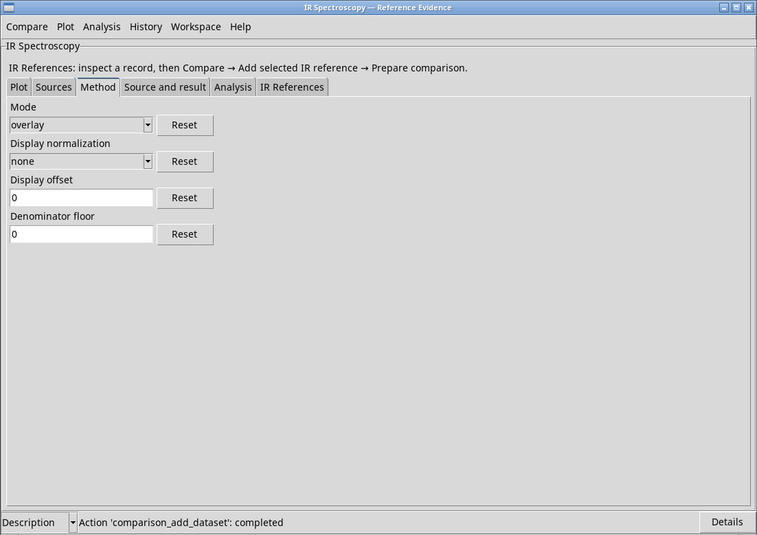
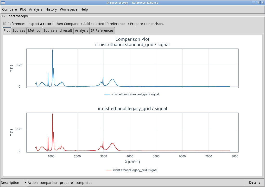
Open Method and choose Mode. Click Compare → Prepare comparison after setting the method and sources. Source and result shows mode, display processing, domain, and missing values. The comparison appears in Plot.
- overlay
- The default mode. It overlays curves on the same axes while retaining the original samples. Use comparable representations for quantitative interpretation.
- top_bottom
- Displays traces in panels with a shared X axis and independent Y axes. Use it to compare shapes whose Y scales or representations differ, as long as their X coordinates are physically compatible.
- stacked
- Overlays traces with a vertical offset. Display offset sets the per-trace increment, initially 0. The offset is a display change expressed on the displayed Y scale.
- difference
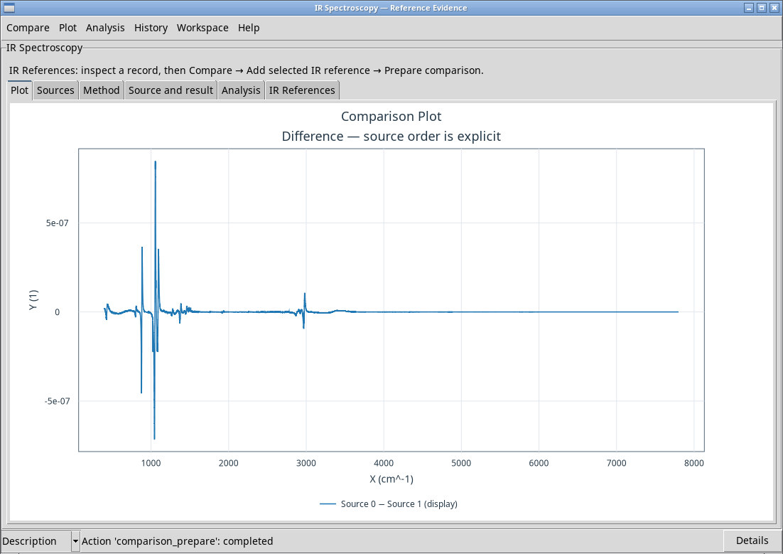
- Subtracts the second comparable source from the first. For sources at positions 0 and 1, the comparison uses the first source’s grid over the common range and linearly interpolates the second. Points outside the overlap are excluded.
- ratio
- Divides the first source by the second over their common domain. In Denominator floor, set the limit for the absolute value of the denominator. The default is 0. Samples that fail the test appear as gaps and are counted in the status.
Display normalization offers none to keep the available scale and minmax to compare shapes on a relative 0–1 scale. Display normalization changes the displayed amplitude. For a quantitative difference or ratio, use none and check that the application accepts the quantities. Reset restores the default for its field.
Interpret a difference or a ratio
The canonical Y values for NIST/PNNL ethanol match sample for sample. The standard and legacy X grids differ by up to about 0.0000236 cm⁻¹. The derived comparison also depends on interpolation on the working grid, so the coordinate difference and realignment can leave a very small residual.