Five verified procedures
PNNL, RefIMP, a comparison across formats, and restoring a saved view.
1. View PNNL ethanol directly from the Library
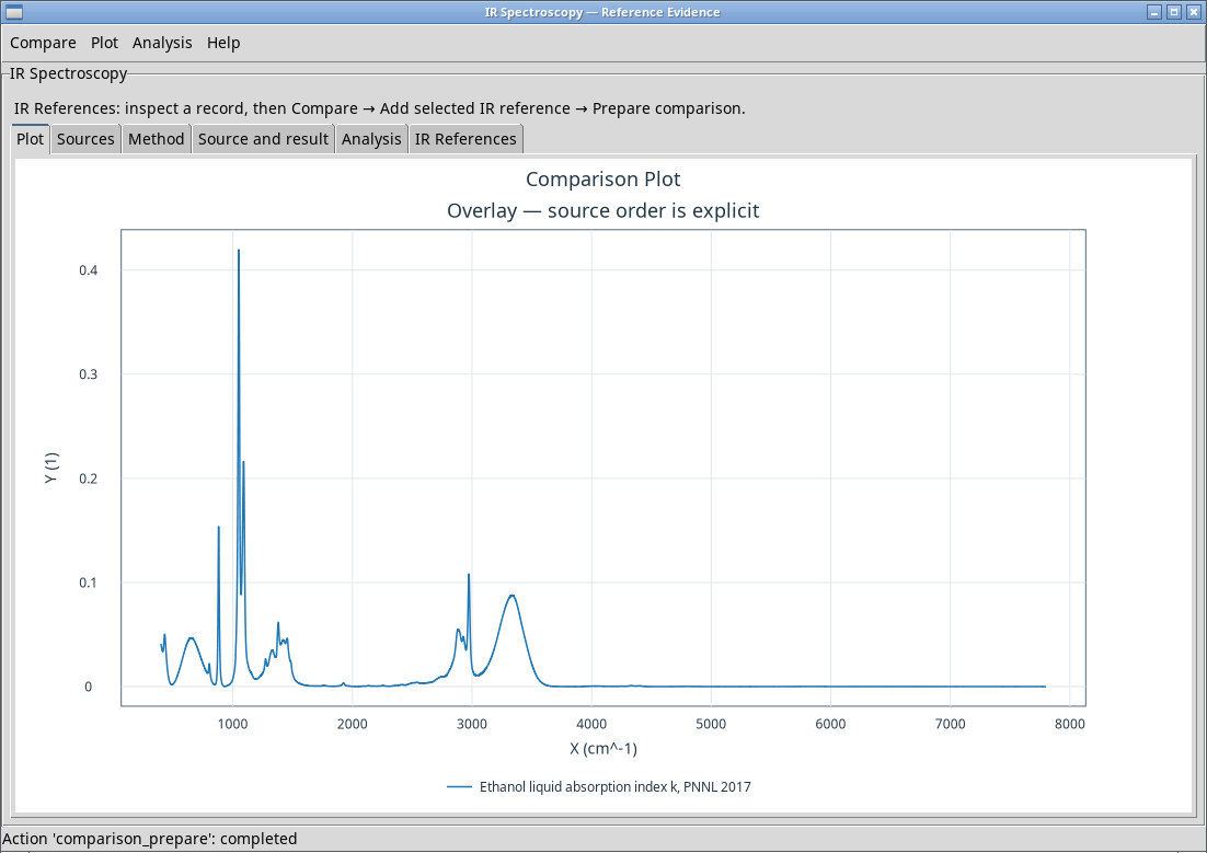
- Install the NIST/PNNL managed library. Open IR Spectroscopy from Viewers, even without an active session.
- In IR References → Records, search for
ethanol-k-pnnl-2017. Select the record and checkwavenumber, cm⁻¹,absorption_index, unit 1, and 15,347 samples. - Use Compare → Add selected IR reference. In Method, choose
overlayandnoneand prepare the plot.
2. Compare two grids for the same optical constant
- Generate and reopen the session with
nist_pnnl_ir_faculty. Addir.nist.ethanol.standard_gridandir.nist.ethanol.legacy_gridto Sources in that order, usingwavenumberandsignal. - Prepare
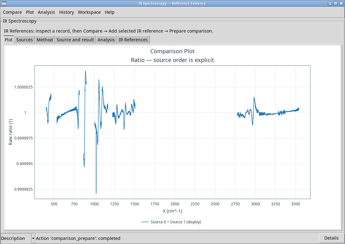
overlay. The two curves overlap almost entirely. Choosedifferenceto inspect the residual from realignment andratioto check the common domain. - In ratio mode, try setting Denominator floor to
0.01and leave Display normalization atnone. Check the missing sample count in Source and result.
3. Verify the same ItemID in HDF5 and CSV
- Generate and reopen the Session with
refimp_full_training_ir. Addir.refimp.item13andir.refimp.csv_compatusingwavenumberandsignal. - Prepare
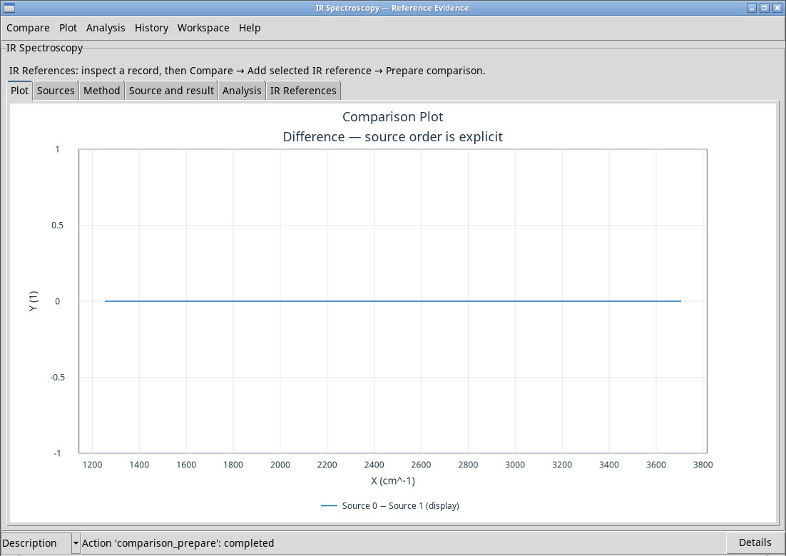
overlayanddifferencewithnone. The 637 pairs agree. The difference confirms that both formats yield equivalent readings of the same ItemID.
RefIMP data by Jana Weisser and Teresa Pohl, 2022, CC BY-SA 4.0. The comparison uses two conversions of the same ItemID. mediaTUM source.
4. Run retrieval against the full RefIMP corpus
- In Analysis → Input, select
ir.refimp.item13and discover its variables. Setwavenumber,signal,relative_transmission_signal, and thetum.refimp.ftir.training.2022Library. - In Processing, use
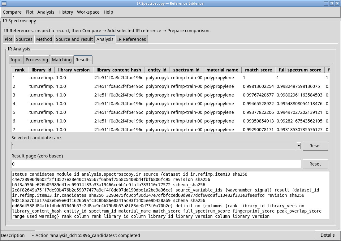
nonefor baseline and smoothing, derivative order 0,mean_center_unit_vector, and a step of 4 cm⁻¹. In Matching, choosecosineand set the band to 1300–1800 cm⁻¹ with a weight of 0.35. Use Run Analysis. - When the results are published, use Read ranked references. The first row is
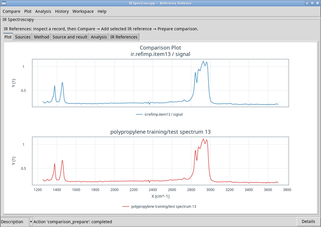
refimp-train-00013with a score of 1.0. This retrieves ItemID 13 from the corpus that contains it. - Keep one measured trace in Sources. In Analysis → Results, choose rank 1 and use Add selected ranked reference. Prepare
top_bottomto view both traces with independent Y axes.
5. Reuse a formatted plot
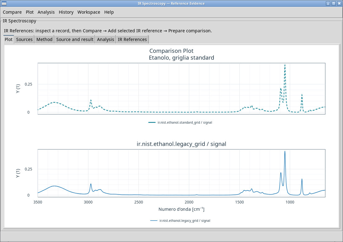
- With both NIST grids in
top_bottom, use Plot → Properties… to set a shared X range of 650–3500 cm⁻¹ and a title for the first panel. - In Series style…, set the first curve to color
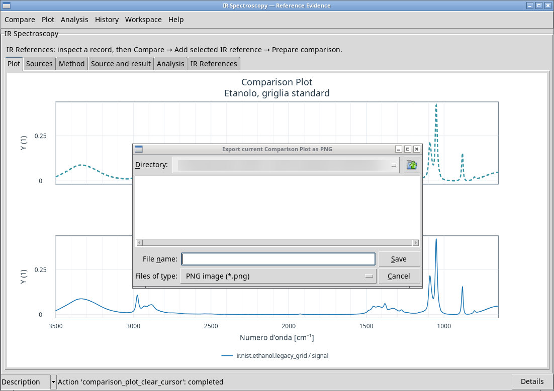
#087C8F, line styledashed, and width 2.5. Apply the changes and save the NIST k due pannelli variant with Save Plot Variant…. - Use Export PNG… to save the result as an image. If you change the view later, use Load Plot Variant… to restore the saved presentation and source selection.