OpenFOAM 14 Case 06: Sensitivity to the Inlet Boundary Condition

Sixth case of the Learning OpenFOAM 14 path, after parallel execution with MPI: sensitivity to inlet boundary conditions — controlled variation of inlet velocity, velocity-profile validation and pressure-gradient verification.

1. Learning objectives

This exercise introduces sensitivity to boundary conditions in CFD. The geometry, mesh, fluid properties and numerical methods are kept fixed while only the inlet velocity is changed.

This is an important modelling concept: a boundary condition is not merely a numerical option. It is part of the mathematical definition of the physical problem. Changing a boundary condition means asking the solver to solve a different physical case.

At the end of this exercise you should be able to:

• identify which parts of a CFD case must remain unchanged in a controlled sensitivity study;
• modify a fixedValue inlet velocity in OpenFOAM;
• run several otherwise identical cases;
• compare velocity profiles against an analytical solution;
• extract and fit a pressure gradient from OpenFOAM results;
• explain why the maximum velocity and pressure gradient scale with the inlet velocity;
• distinguish a physical sensitivity from a mesh or solver effect.

2. Reference geometry and numerical model

This exercise reuses the validated parametric channel from CFD Training Case 04.

Quantity	Value
Channel length	0.75 m
Channel gap	0.015 m
Channel depth	0.001 m
Mesh	300 × 60 × 1
Total cells	18,000
Cell type	hexahedra
Kinematic viscosity	1.0e-6 m²/s
Solver module	incompressibleFluid via foamRun
Flow model	laminar

The mesh and all numerical settings are kept identical in the three cases.

3. What is changed, and what is not changed

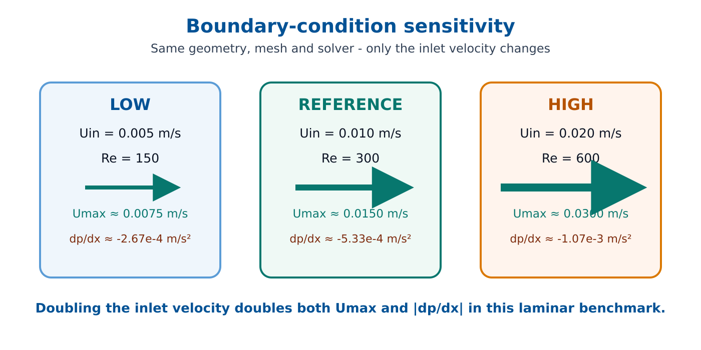
Three inlet velocities are investigated:

Case	Mean inlet velocity [m/s]	Reynolds number	Analytical maximum velocity [m/s]
low	0.005	150	0.0075
reference	0.010	300	0.0150
high	0.020	600	0.0300

The following items must remain identical:

• geometry;
• mesh;
• viscosity;
• outlet pressure condition;
• wall condition;
• fvSchemes;
• fvSolution;
• solver;
• post-processing location.

Only the inlet value in 0/U is changed.

4. Expected analytical behaviour

For fully developed laminar flow between parallel plates,

U_max = 1.5 U_mean.

Therefore, if the inlet mean velocity is doubled, the fully developed maximum velocity must also double.

For a channel gap H, the kinematic pressure gradient is

dp/dx = −12 ν U_mean / H².

In this exercise, H = 0.015 m and ν = 10⁻⁶ m²/s. The theoretical pressure gradients are therefore:

Case	Theoretical dp/dx [m/s²]
low	-2.6666667e-4
reference	-5.3333333e-4
high	-1.0666667e-3

The pressure variable in this incompressible OpenFOAM formulation is kinematic pressure, i.e. pressure divided by density. For water, a kinematic pressure difference can be converted approximately to pascals by multiplying by the density.

5. Prerequisites

The validated Case 04 directory must exist:

$FOAM_RUN/04_parametric_channel

Check the main commands:

foamVersion
command -v checkMesh
command -v foamRun
command -v foamPostProcess

Expected OpenFOAM version:

14

6. Create the three sensitivity cases

Create three copies of the validated case:

cd $FOAM_RUN

mkdir -p 06_boundary_sensitivity/{low,reference,high}

for c in low reference high; do
    cp -a 04_parametric_channel/0 \
          06_boundary_sensitivity/$c/

    cp -a 04_parametric_channel/constant \
          06_boundary_sensitivity/$c/

    cp -a 04_parametric_channel/system \
          06_boundary_sensitivity/$c/

    rm -rf \
      06_boundary_sensitivity/$c/constant/polyMesh_reference
done

The resulting directory structure is:

06_boundary_sensitivity/
|-- low/
|   |-- 0/
|   |-- constant/
|   `-- system/
|-- reference/
|   |-- 0/
|   |-- constant/
|   `-- system/
`-- high/
    |-- 0/
    |-- constant/
    `-- system/

7. Modify only the inlet boundary condition

The reference case already uses 0.010 m/s.

For the low case:

sed -i \
's/value[[:space:]]*uniform (0.01 0 0);/value            uniform (0.005 0 0);/' \
06_boundary_sensitivity/low/0/U

For the high case:

sed -i \
's/value[[:space:]]*uniform (0.01 0 0);/value            uniform (0.020 0 0);/' \
06_boundary_sensitivity/high/0/U

Check all three inlet definitions:

for c in low reference high; do
    echo "===== $c ====="
    grep -A4 "inlet" \
      06_boundary_sensitivity/$c/0/U
done

Expected values:

low       -> (0.005 0 0)
reference -> (0.010 0 0)
high      -> (0.020 0 0)

The inlet boundary condition is a fixedValue because the velocity is directly prescribed.

8. Confirm that the mesh is unchanged

A sensitivity study is meaningful only if the controlled variable is actually isolated. Check every case:

for c in low reference high; do
    echo "===== $c ====="

    cd $FOAM_RUN/06_boundary_sensitivity/$c

    checkMesh > log.checkMesh

    grep -E \
    'cells:|hexahedra:|Mesh OK' \
    log.checkMesh
done

Expected output for every case:

cells:       18000
hexahedra:   18000
Mesh OK.

If the cell count differs between cases, the study is no longer a pure boundary-condition sensitivity test.

9. Run the three calculations

Run all three cases while measuring wall time:

cd $FOAM_RUN/06_boundary_sensitivity

for c in low reference high; do

    echo
    echo "=========================="
    echo "Running $c"
    echo "=========================="

    cd $FOAM_RUN/06_boundary_sensitivity/$c

    /usr/bin/time \
        -o log.time \
        -f 'Wall time: %e s' \
        foamRun > log.foamRun 2>&1

    tail -3 log.foamRun
    cat log.time

done

A successful run ends with:

End

Measured wall times were:

Case	Wall time [s]
low	143.05
reference	143.68
high	141.63

The times are nearly equal because the mesh size, solver and number of steady iterations are nearly the same. Changing the inlet value does not by itself create a larger computational problem.

10. Velocity-profile post-processing

The transverse sampling line is inherited from Case 04 and is located near the outlet, where the flow is fully developed.

The corresponding system/graphUniform should contain:

FoamFile
{
    format        ascii;
    class         dictionary;
    object        graphUniform;
}

start             (0.675 -0.007375 0.0005);
end               (0.675 0.007375 0.0005);

nPoints           201;

fields            (U);

axis              y;

#includeEtc "caseDicts/postProcessing/graphs/graphUniform.cfg"

Extract the profile for all cases:

for c in low reference high; do

    cd $FOAM_RUN/06_boundary_sensitivity/$c

    foamPostProcess \
        -solver incompressibleFluid \
        -func graphUniform \
        -latestTime

done

The output is written under:

postProcessing/graphUniform/<time>/line.xy

11. Automatic velocity validation

Return to the common directory:

cd $FOAM_RUN/06_boundary_sensitivity

Define the analysis function:

analyse_case()
{
    CASE=$1
    UMEAN=$2

    FILE=$(find "$CASE/postProcessing/graphUniform" \
        -name line.xy | sort -V | tail -1)

    awk \
    -v CASE="$CASE" \
    -v Umean="$UMEAN" '
    BEGIN {
        H=0.015
        UmaxTheory=1.5*Umean
        umax=-1
    }

    $1 !~ /^#/ && NF >= 2 {

        y=$1
        u=$2

        uth=UmaxTheory*(1-(2*y/H)^2)

        e=u-uth
        ae=(e<0 ? -e : e)

        sumsq += e*e
        n++

        if (ae > maxerr)
            maxerr=ae

        if (u > umax)
            umax=u
    }

    END {
        rmse=sqrt(sumsq/n)

        printf "%-10s %10.5f %14.9f %14.9f %12.6f %12.6f\n",
               CASE,
               Umean,
               umax,
               UmaxTheory,
               100*rmse/UmaxTheory,
               100*maxerr/UmaxTheory
    }' "$FILE"
}

Print the table header and analyse the three cases:

printf "%-10s %10s %14s %14s %12s %12s\n" \
"CASE" "UMEAN" "UMAX_CFD" "UMAX_THEORY" "NRMSE_%" "MAXERR_%"

analyse_case low       0.005
analyse_case reference 0.010
analyse_case high      0.020

12. Measured velocity results

The measured results are:

Case	Umean [m/s]	Umax,CFD [m/s]	Umax,theory [m/s]	NRMSE [%]	Max error [%]
low	0.00500	0.007495834	0.007500000	0.058847	0.083101
reference	0.01000	0.014991664	0.015000000	0.058850	0.083131
high	0.02000	0.029983232	0.030000000	0.058886	0.083441

The CFD maximum velocity scales almost exactly with the imposed inlet velocity.

The direct errors in U_max relative to the analytical value are approximately:

Case	Relative error in Umax [%]
low	0.05555
reference	0.05557
high	0.05589

The normalized profile error remains almost unchanged. This is expected because the same mesh and numerical discretization are used in all three calculations.

13. Why the velocity result is linear

For this laminar benchmark, the governing equations and boundary conditions produce a velocity field that scales linearly with the imposed mean velocity.

For parallel-plate Poiseuille flow:

U_max = 1.5 U_mean.

Therefore:

Umean:     0.005 -> 0.010 -> 0.020 m/s
Umax:    ~ 0.0075 -> 0.0150 -> 0.0300 m/s

The shape of the normalized parabola does not change. Only its amplitude changes.

14. Pressure-gradient post-processing

Velocity is only one consequence of changing the inlet boundary condition. The pressure gradient required to drive the fully developed flow must also change.

Create system/graphPressure in every case:

cd $FOAM_RUN/06_boundary_sensitivity

for c in low reference high; do

cat > $c/system/graphPressure <<'EOF2'
FoamFile
{
    format      ascii;
    class       dictionary;
    object      graphPressure;
}

start           (0.55 0 0.0005);
end             (0.70 0 0.0005);

nPoints         101;

fields          (p);

axis            x;

#includeEtc "caseDicts/postProcessing/graphs/graphUniform.cfg"
EOF2

done

The line is placed in the downstream region so that the pressure gradient is measured where the flow is already developed.

Extract the pressure samples:

for c in low reference high; do

    cd $FOAM_RUN/06_boundary_sensitivity/$c

    foamPostProcess \
        -solver incompressibleFluid \
        -func graphPressure \
        -latestTime

done

15. Compute the pressure gradient by linear regression

The pressure field should be approximately linear with x in the fully developed region. Instead of using only two points, fit all 101 samples with a straight line.

Return to the common directory:

cd $FOAM_RUN/06_boundary_sensitivity

Define:

pressure_slope()
{
    CASE=$1

    FILE=$(find "$CASE/postProcessing/graphPressure" \
        -name line.xy | sort -V | tail -1)

    awk -v CASE="$CASE" '
    $1 !~ /^#/ && NF >= 2 {
        x=$1
        p=$2

        sx+=x
        sp+=p
        sxx+=x*x
        sxp+=x*p
        n++
    }

    END {
        slope=(n*sxp-sx*sp)/(n*sxx-sx*sx)

        printf "%-10s %.10e\n", CASE, slope
    }' "$FILE"
}

Then run:

printf "%-10s %18s\n" "CASE" "CFD dp/dx"
pressure_slope low
pressure_slope reference
pressure_slope high

16. Measured pressure-gradient results

The measured gradients are:

Case	CFD dp/dx [m/s²]	Theory [m/s²]	Relative error [%]
low	-2.6651869423e-4	-2.6666667e-4	0.05549
reference	-5.3303768616e-4	-5.3333333e-4	0.05543
high	-1.0661283532e-3	-1.0666667e-3	0.05047

The scaling is also correct:

(dp/dx)_reference / (dp/dx)_low ≈ 2.00000

and

(dp/dx)_high / (dp/dx)_reference ≈ 2.00010.

Thus, within numerical error, doubling the inlet velocity doubles the magnitude of the pressure gradient.

17. Interpreting the complete result

This sensitivity study establishes three important points.

17.1 The boundary condition changes the physical solution

The three cases use the same numerical method, but they do not represent the same physical state. The different inlet velocities produce different velocity amplitudes and different pressure gradients.

17.2 The numerical error remains stable

The velocity-profile NRMSE remains close to 0.059% in all three cases. This indicates that the discretization quality is similar across the tested range.

17.3 Computational cost remains similar

The measured wall times are all close to 142–144 seconds. The problem size has not changed: there are still 18,000 cells and the same steady solution process is used.

This is a useful distinction:

change in physical input   -> different physical result
same mesh and solver       -> similar numerical cost

18. Optional ParaView comparison

A visual comparison is optional because the quantitative validation is already conclusive. If desired, create a .foam file in each case:

touch low/low.foam
touch reference/reference.foam
touch high/high.foam

Open the three cases in ParaView and compare U → Magnitude.

For a meaningful visual comparison, use the same colour range for all three datasets. If each dataset is automatically rescaled independently, the three fields may look deceptively similar even though their absolute velocities differ by factors of two and four.

The streamline geometry remains straight in all cases; only the velocity magnitude changes. Therefore, streamline shape is not the primary result of this exercise.

19. Acceptance criteria

Case 06 is complete when all of the following are satisfied:

• the three cases contain exactly 18,000 hexahedral cells;
• checkMesh reports Mesh OK for each case;
• the only controlled change is the inlet fixedValue velocity;
• all three calculations finish normally;
• the maximum velocity agrees with 1.5 U_mean;
• the normalized velocity-profile error remains small;
• the measured pressure gradient agrees with the analytical value;
• doubling the inlet velocity approximately doubles both U_max and |dp/dx|.

20. Common checks if the result is unexpected

If all three cases give the same velocity field:

1. inspect 0/U in each case;
2. confirm that the inlet value is actually different;
3. verify that the solver was run separately in each directory;
4. check that post-processing reads the correct case and latest time.

If the pressure-gradient file is missing:

1. confirm that system/graphPressure exists;
2. confirm that fields (p); is present;
3. rerun foamPostProcess -func graphPressure -latestTime.

If checkMesh gives different cell counts between cases, recreate the three cases from the same validated source before continuing.

21. Review questions

After completing the exercise, you should be able to answer:

1. Why must geometry and mesh remain identical in this sensitivity study?
2. Why is the inlet velocity a physical input rather than merely a numerical parameter?
3. Why does U_max double when U_mean doubles in this laminar benchmark?
4. Why does the pressure-gradient magnitude also double?
5. Why do the three calculations require almost the same execution time?
6. Why is it misleading to compare three ParaView images if each image uses an automatically rescaled colour range?

22. Final conclusion

This exercise demonstrates a controlled CFD sensitivity study. By varying only the inlet velocity, the effect of the boundary condition is isolated from mesh and solver effects.

The measured velocity fields and pressure gradients follow the analytical Poiseuille scaling with errors of approximately 0.05–0.06%. The exercise therefore confirms both the physical interpretation of the boundary condition and the numerical consistency of the OpenFOAM solution.

This closes the first introductory block of the Learning OpenFOAM 14 path. Previous case: parallel execution with MPI, decomposePar and reconstructPar.