OpenFOAM 14 Case 05: Parallel Runs with MPI, decomposePar and reconstructPar

Fifth case of the Learning OpenFOAM 14 path: parallel runs with MPI. The parametric channel validated in Case 04 is solved twice, once in serial with a single process and once after splitting the mesh into four subdomains, with four MPI processes.

CFD Training Case 05 – Parallel OpenFOAM Execution with MPI. OpenFOAM 14: domain decomposition, parallel execution, reconstruction and numerical equivalence.

1. Learning objectives

This exercise introduces parallel CFD execution with MPI in OpenFOAM 14. A previously validated channel case is run twice:

1. once as a normal serial calculation using one OpenFOAM process;
2. once after decomposing the mesh into four subdomains and running four MPI processes.

The exercise is not only about obtaining a shorter execution time. The student must also verify that the parallel calculation produces the same physical solution as the serial calculation.

At the end of this exercise the student should be able to:

• explain why a CFD domain can be divided among several processes;
• create a decomposeParDict file;
• use the scotch decomposition method;
• run decomposePar;
• launch OpenFOAM with mpirun and the -parallel option;
• reconstruct the distributed result using reconstructPar;
• compare serial and parallel results quantitatively;
• calculate speed-up and parallel efficiency;
• understand why parallel execution is not always exactly proportional to the number of processes.

2. Reference case

The reference case is the validated parametric channel from CFD Training Case 04.

Quantity	Value
Channel length	0.75 m
Channel gap	0.015 m
Channel depth	0.001 m
Mesh	300 × 60 × 1
Total cells	18,000
Cell type	hexahedra
Mean inlet velocity	0.010 m/s
Kinematic viscosity	1.0e-6 m²/s
Reynolds number	300
Analytical maximum velocity	0.015 m/s

The Case 04 numerical validation gave:

• CFD maximum velocity: 0.0149916640 m/s;
• normalized RMSE against the analytical profile: 0.058850%;
• maximum pointwise error relative to the analytical maximum: 0.083131%.

This already validated solution is used so that only the execution mode changes in Case 05.

3. What MPI changes

In a serial run, one process owns the complete mesh and solves all equations.

In a parallel run, OpenFOAM divides the mesh into subdomains. Each MPI process owns one subdomain and exchanges information with neighboring processes across processor boundaries.

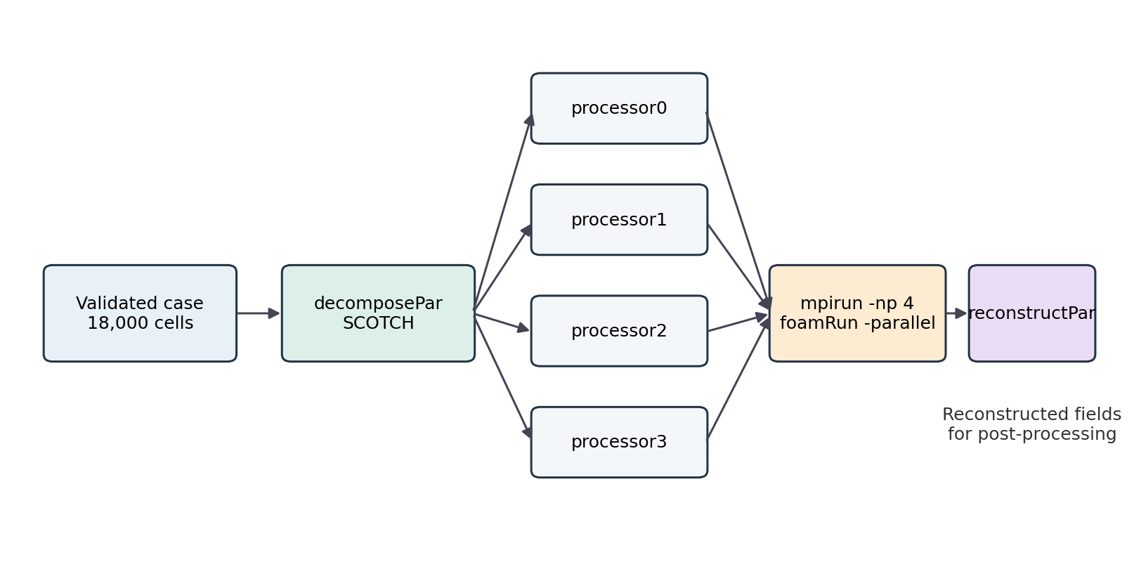
The main sequence is:

complete case
    |
    v
decomposePar
    |
    +--> processor0
    +--> processor1
    +--> processor2
    +--> processor3
            |
            v
     foamRun -parallel
            |
            v
      reconstructPar
            |
            v
complete reconstructed result

The physics is unchanged. Only the numerical workload is distributed among multiple processes.

4. Prerequisites

OpenFOAM 14 and OpenMPI must already be working.

Check the required commands:

foamVersion
command -v foamRun
command -v decomposePar
command -v reconstructPar
command -v mpirun

Expected OpenFOAM version:

14

A simple MPI check can also be made with:

mpirun --version

This exercise uses four MPI processes. The machine must therefore provide at least four CPU execution contexts for a meaningful test.

5. Create the serial and parallel cases

Start from the validated Case 04 directory:

$FOAM_RUN/04_parametric_channel

Create two clean copies containing the same initial fields, mesh and numerical settings:

cd $FOAM_RUN

mkdir -p 05_parallel_channel/{serial,parallel}

for c in serial parallel; do
    cp -a 04_parametric_channel/0          05_parallel_channel/$c/
    cp -a 04_parametric_channel/constant   05_parallel_channel/$c/
    cp -a 04_parametric_channel/system     05_parallel_channel/$c/

    rm -rf 05_parallel_channel/$c/constant/polyMesh_reference
done

The resulting structure is:

05_parallel_channel/
|-- serial/
|   |-- 0/
|   |-- constant/
|   `-- system/
`-- parallel/
    |-- 0/
    |-- constant/
    `-- system/

The two cases must be identical before decomposition.

6. Serial reference run

The serial calculation provides the reference execution time and reference numerical solution.

Enter the serial directory:

cd $FOAM_RUN/05_parallel_channel/serial

Run OpenFOAM while measuring the real elapsed wall time:

/usr/bin/time \
    -o log.time.serial \
    -f 'Serial wall time: %e s' \
    foamRun > log.foamRun 2>&1

The solver output is redirected to log.foamRun. During execution it can be monitored from a second terminal with:

tail -f log.foamRun

A successful calculation finishes with:

End

Check the final lines and measured time:

tail -10 log.foamRun
cat log.time.serial

Measured result for this exercise:

Serial wall time: 144.37 s

The OpenFOAM log at the final iteration contained:

Time = 2000s
DICPCG: Solving for p, Initial residual = 1.6999328e-10,
Final residual = 7.3423107e-11, No Iterations 260
ExecutionTime = 144.16033 s ClockTime = 144 s
End

The value printed as Time = 2000s is the steady-run iteration/time label used by this case, not the measured elapsed runtime. The end-to-end wall time is taken from /usr/bin/time.

7. Serial post-processing

Extract the reference velocity profile:

foamPostProcess \
    -solver incompressibleFluid \
    -func graphUniform \
    -latestTime

The expected file is typically:

postProcessing/graphUniform/2000/line.xy

It contains the sampled cross-channel velocity profile used later for the serial/parallel comparison.

8. Parallel configuration: decomposeParDict

Enter the parallel case:

cd $FOAM_RUN/05_parallel_channel/parallel

Create system/decomposeParDict:

cat > system/decomposeParDict <<'EOF'
FoamFile
{
    format      ascii;
    class       dictionary;
    object      decomposeParDict;
}

numberOfSubdomains 4;

method scotch;
EOF

The important entries are:

• numberOfSubdomains 4; – create four computational subdomains;
• method scotch; – let SCOTCH partition the mesh automatically.

8.1 Why use SCOTCH?

A good domain decomposition should achieve two goals:

1. give approximately the same amount of work to every process;
2. minimize interfaces between processes, because data crossing those interfaces requires MPI communication.

SCOTCH treats the mesh connectivity as a graph and automatically finds a useful partition. This makes it a good general-purpose choice when no special geometric decomposition is required.

9. Decompose the mesh

Run:

decomposePar | tee log.decomposePar

The case should now contain:

processor0/
processor1/
processor2/
processor3/

Verify:

ls -d processor*

Check the cell distribution:

grep -E "Processor [0-9]|Number of cells" log.decomposePar

Measured decomposition:

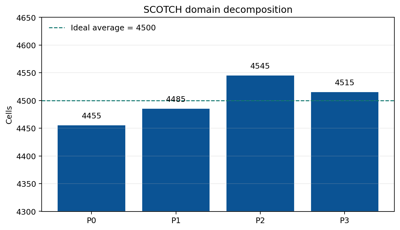
Processor 0
    Number of cells = 4455
Processor 1
    Number of cells = 4485
Processor 2
    Number of cells = 4545
Processor 3
    Number of cells = 4515

The ideal average is:

18000 / 4 = 4500 cells/process

The actual distribution is therefore very well balanced.

The smallest subdomain contains 4455 cells and the largest 4545 cells. The full range is only 90 cells, equal to 2% of the ideal 4500-cell share.

10. Run with four MPI processes

Launch the parallel calculation:

/usr/bin/time \
    -o log.time.parallel \
    -f 'Parallel wall time: %e s' \
    mpirun -np 4 foamRun -parallel > log.foamRun 2>&1

The important elements are:

• mpirun -np 4 starts four MPI processes;
• foamRun executes the solver;
• -parallel tells OpenFOAM to use the decomposed case.

Monitor the calculation if required:

tail -f log.foamRun

A successful parallel run finishes with:

End
Finalising parallel run

Check the final lines and wall time:

tail -10 log.foamRun
cat log.time.parallel

Measured result:

Parallel wall time: 40.95 s

The final OpenFOAM output included:

Time = 2000s
DICPCG: Solving for p, Initial residual = 1.8497959e-10,
Final residual = 8.9784387e-11, No Iterations 265
time step continuity errors : sum local = 8.2197286e-13,
global = 6.4830667e-15, cumulative = -4.7805998e-07
ExecutionTime = 40.664163 s ClockTime = 41 s
End
Finalising parallel run

11. Reconstruct the parallel result

After a parallel calculation, each processorN directory contains only its local part of the solution. Many normal post-processing operations are easier after rebuilding the complete fields.

Run:

reconstructPar | tee log.reconstructPar

reconstructPar combines the distributed processor fields into normal time directories in the main case. The processor directories are not deleted automatically. They can be kept as evidence of the parallel calculation or removed later after reconstruction has been verified.

12. Parallel post-processing

After reconstruction, extract the same velocity profile used for the serial case:

foamPostProcess \
    -solver incompressibleFluid \
    -func graphUniform \
    -latestTime

The serial and parallel cases should now both contain a line.xy profile generated using identical sampling coordinates.

13. Quantitative serial/parallel comparison

Move to the parent directory:

cd $FOAM_RUN/05_parallel_channel

Locate the final profiles:

S=$(find serial/postProcessing/graphUniform \
    -name line.xy | sort -V | tail -1)

P=$(find parallel/postProcessing/graphUniform \
    -name line.xy | sort -V | tail -1)

echo "$S"
echo "$P"

Compare the two profiles point by point:

paste \
    <(grep -v '^#' "$S") \
    <(grep -v '^#' "$P") |
awk '
{
    ys=$1
    us=$2

    yp=$5
    up=$6

    d=up-us
    ad=(d<0 ? -d : d)

    sumsq += d*d
    n++

    if (ad > maxdiff) {
        maxdiff=ad
        maxy=ys
    }

    if (us > umaxS)
        umaxS=us

    if (up > umaxP)
        umaxP=up
}
END {
    rmse=sqrt(sumsq/n)

    printf "Points                   : %d\n",n
    printf "Serial Umax              : %.12f m/s\n",umaxS
    printf "Parallel Umax            : %.12f m/s\n",umaxP

    printf "Profile RMSE S vs P      : %.12e m/s\n",rmse
    printf "Maximum abs difference   : %.12e m/s\n",maxdiff
    printf "Max-difference y         : %.8f m\n",maxy

    printf "Max diff / 0.015         : %.12e %%\n",
           100*maxdiff/0.015
}'

Measured result:

Points                   : 201
Serial Umax              : 0.014991664000 m/s
Parallel Umax            : 0.014991664000 m/s
Profile RMSE S vs P      : 1.577200743861e-11 m/s
Maximum abs difference   : 1.000000004678e-10 m/s
Max-difference y         : -0.00545750 m
Max diff / 0.015         : 6.666666697852e-07 %

The serial and parallel maximum velocities are identical to the displayed precision.

The maximum difference between the two sampled profiles is approximately

1 × 10⁻¹⁰ m/s

which is negligible compared with the characteristic velocity of 0.015 m/s.

14. Why tiny differences can still appear

Floating-point arithmetic is not perfectly associative. In other words,

(a + b) + c

and

a + (b + c)

can differ in their last binary digits when finite-precision arithmetic is used.

In a parallel calculation, MPI reductions and the decomposition of matrix operations can change the order in which additions and other floating-point operations are performed. Therefore, a parallel solution should not always be expected to be bit-for-bit identical to a serial solution.

The correct requirement is that the differences are numerically insignificant relative to the accuracy required by the physical problem.

In this exercise the observed difference is many orders of magnitude smaller than the discretization error of the CFD solution itself.

15. Speed-up

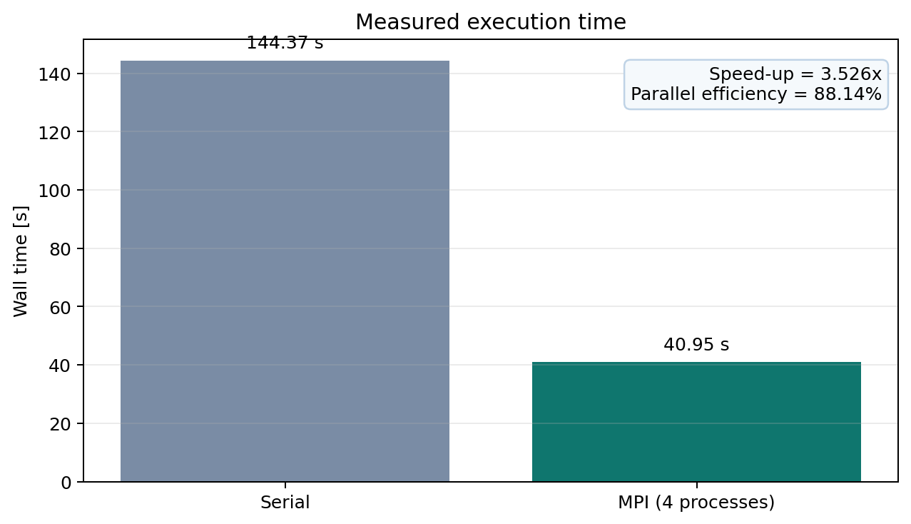
The measured wall times are:

Execution mode	Wall time
Serial	144.37 s
MPI, 4 processes	40.95 s

The parallel speed-up is defined as

S_p = T₁ / T_p

where T₁ is the serial wall time and T_p is the wall time using p processes.

For this case:

S₄ = 144.37 / 40.95 = 3.526

Thus the four-process calculation is approximately 3.53 times faster than the serial calculation.

16. Parallel efficiency

Parallel efficiency describes how effectively the available processes are used:

η_p = S_p / p

For four processes:

η₄ = 3.526 / 4 = 0.8814

or

η₄ = 88.14%

This is a strong result for this test case.

The wall-time reduction is:

(144.37 − 40.95) / 144.37 × 100 = 71.64%

17. Why speed-up is not exactly four

An ideal four-process calculation would require exactly one quarter of the serial time:

T_ideal = 144.37 / 4 = 36.09 s

The measured parallel time is 40.95 s. The additional time comes from parallel overhead, including:

• MPI communication across processor boundaries;
• synchronization between processes;
• decomposition-related interface operations;
• startup and coordination overhead;
• parts of the algorithm that cannot be perfectly divided.

As the number of processes increases, communication normally becomes more important. Therefore, doubling the number of MPI processes does not automatically halve the runtime.

For very small meshes, parallel execution can even be slower than serial execution. For very large CFD cases, however, parallel execution is often essential both for runtime and for distributing memory requirements.

18. Automatic performance calculation

The measured wall times can be converted into speed-up and efficiency directly from the log files:

serial=$(awk '{print $4}' serial/log.time.serial)
parallel=$(awk '{print $4}' parallel/log.time.parallel)

awk -v ts="$serial" -v tp="$parallel" '
BEGIN {
    p=4
    speedup=ts/tp
    efficiency=100*speedup/p
    reduction=100*(ts-tp)/ts

    printf "Serial wall time      : %.2f s\n",ts
    printf "Parallel wall time    : %.2f s\n",tp
    printf "Speed-up              : %.3f x\n",speedup
    printf "Parallel efficiency   : %.2f %%\n",efficiency
    printf "Wall-time reduction   : %.2f %%\n",reduction
}'

Expected output for this exercise:

Serial wall time       : 144.37 s
Parallel wall time     : 40.95 s
Speed-up               : 3.526 x
Parallel efficiency    : 88.14 %
Wall-time reduction    : 71.64 %

19. Optional ParaView check

A new visualization is not required to validate the parallel algorithm because the point-by-point numerical comparison is much more stringent.

If a visual check is desired, create a .foam marker file in the reconstructed parallel case:

cd $FOAM_RUN/05_parallel_channel/parallel
touch parallel_channel.foam

Connect with the ParaView client through pvserver, open the reconstructed case, and verify U and p at the final time.

The visual result should be indistinguishable from the serial Case 04 solution.

20. Acceptance criteria

The exercise is complete when all of the following conditions are satisfied:

• the serial run reaches End;
• decomposePar creates four processorN directories;
• the SCOTCH decomposition distributes the cells reasonably evenly;
• the MPI run reaches End and Finalising parallel run;
• reconstructPar completes successfully;
• serial and parallel velocity maxima agree;
• the serial/parallel profile difference is negligible compared with the CFD discretization error;
• serial and parallel wall times are measured using the same method;
• speed-up and efficiency are calculated and interpreted.

For the measured test:

Criterion	Result
Serial wall time	144.37 s
4-process wall time	40.95 s
Speed-up	3.526 x
Parallel efficiency	88.14%
Serial Umax	0.014991664000 m/s
Parallel Umax	0.014991664000 m/s
Maximum profile difference	1.0e-10 m/s
Numerical equivalence	PASS

21. Final conclusion

This exercise demonstrates the complete OpenFOAM parallel workflow:

validated case
    -> decomposePar
    -> MPI execution
    -> reconstructPar
    -> quantitative comparison

The four-process run reduced wall time from 144.37 s to 40.95 s, giving a measured speed-up of 3.526 and a parallel efficiency of 88.14%.

More importantly, the reconstructed parallel solution is numerically equivalent to the serial solution to approximately 10⁻¹⁰ m/s in the sampled velocity profile.

The key lesson is that parallel CFD must be evaluated using both performance and numerical correctness. A calculation is not successfully parallelized merely because it runs faster: it must also preserve the physical solution.

In Case 06 we go back to serial runs to study sensitivity to the inlet boundary condition.