

OpenFOAM: boundary conditions and physical models in a complete case
Seventh operating guide on OpenFOAM installed on a Linux server and used from Windows, after those on server and transfers, monitoring and convergence, quantitative analysis with ParaView, verification and validation, parameter sweeps and mesh generation. This one connects the mesh to the physical problem: boundary conditions, properties and models in a complete case. The deep-dive boxes open with a click: they contain every package file, the analytic reference solution for the duct with expected numerical values, and verification procedures.
Turning a mesh into a complete, verifiable, reproducible CFD case
Practical handbook · OpenFOAM Foundation 14 · Linux computation, Windows workstation
Edition: October 2026 · Level: intermediate · Original exercise licence: GNU GPL v3 or later.
Goal. Connect geometry, physical properties, initial and boundary conditions, numerical algorithms and measurable results. The accompanying package contains one complete case with three execution modes, always preserving the source templates. Optional background boxes can be skipped by readers familiar with fluid mechanics.
1. From a mesh to a physical problem
A valid mesh does not by itself define a simulation. We must select which equations to solve, which fluid properties to use, which values to impose on each patch, and how to assess whether the results are credible. Boundary conditions are part of the numerical experiment, not merely configuration syntax.
An OpenFOAM case contains 0/ (fields, initial and boundary conditions), constant/ (physical properties and models), system/ (control, discretisation and solution settings), and constant/polyMesh/ after meshing. The present example is steady, laminar, incompressible and isothermal; no temperature or turbulence fields are needed.
Background — governing equations. For a constant-density Newtonian incompressible fluid, continuity requires ∇·U = 0. Momentum conservation combines convection, the pressure gradient and viscous transport. The physical problem is defined by the boundary constraints in addition to the equations themselves.
Deep dive · The equations the incompressibleFluid module actually solves
For a constant-density Newtonian fluid, in kinematic form (divided by ρ):
∇·U = 0
∂U/∂t + ∇·(U U) = −∇p + ∇·[ ν_eff (∇U + (∇U)ᵀ) ]

p = p_phys / ρ      [m²/s²]
ν_eff = ν (laminare)  oppure  ν + ν_t (RAS/LES)
Two practical consequences. First: the solver does not know ρ, so neither pressure nor forces come out in SI units until multiplied by a declared density. Second: in incompressible flow pressure is not a thermodynamic variable but the multiplier enforcing ∇·U = 0; it is therefore defined up to a constant, which is why at least one reference value is needed (here p = 0 at the outlet). The div((nuEff*dev2(T(grad(U))))) term in fvSchemes corresponds to the transposed part of the viscous stress.
Deep dive · A well-posed problem: how many conditions, and where
For incompressible Navier–Stokes, on each portion of the boundary one generally prescribes either velocity (inlets, walls) or a “traction” condition, which OpenFOAM in practice approximates by fixing pressure and a zero velocity gradient (outlets). The proper combination for a duct is therefore: velocity or flow rate at the inlet with zero pressure gradient; fixed pressure at the outlet with zero velocity gradient; no-slip on walls. Prescribing both velocity and pressure on the same patch over-constrains the problem; prescribing pressure nowhere leaves it undetermined.
Deep dive · Why laminar: the dimensionless numbers of the case
In ducts, transition to turbulence occurs under ordinary conditions around Re ≈ 2000–2300 based on the hydraulic diameter; very disturbed inlets can bring it forward, very clean ones can delay it considerably. With Re ≈ 133 the case is laminar by a wide margin. The second number to look at is the ratio of channel length to entrance length, L/L_e ≈ 0.20/0.044 ≈ 4.5: the flow develops and stays developed for about three quarters of the channel, a necessary condition for comparing it with the analytic solution.
2. Version-specific dictionaries: Foundation 14
This handbook targets OpenFOAM Foundation 14, not an OpenCFD/ESI release. In Foundation 14, incompressibleFluid is selected with solver incompressibleFluid; inside system/controlDict and run using foamRun. Kinematic viscosity is defined in constant/physicalProperties using viscosityModel constant; and nu. The momentum transport model is selected in constant/momentumTransport using simulationType laminar;. Copying examples based on transportProperties, turbulenceProperties, application simpleFoam, or different executables can mean mixing incompatible conventions.
Check your installation:
source /opt/OpenFOAM-14/etc/bashrc
foamVersion
command -v foamRun
Rule: after changing OpenFOAM distributions or versions, start with the tutorials belonging to that installation and compare every dictionary. The files provided with this handbook never modify your OpenFOAM installation.
Deep dive · Foundation vs OpenCFD: the differences you meet immediately
| Aspect | OpenFOAM Foundation 14 | OpenCFD/ESI and older Foundation releases |
|---|---|---|
| launch | foamRun with solver incompressibleFluid; | simpleFoam, pimpleFoam (application) |
| viscosity | constant/physicalProperties | constant/transportProperties |
| turbulence | constant/momentumTransport | constant/turbulenceProperties |
| algorithm | dictionary PIMPLE also for steady cases | SIMPLE / PIMPLE |
| version | foamVersion → 14 | foamVersion or log banner |
The quickest check is to read the banner of any log and compare file names with those of the installed tutorial. An extra dictionary does not always produce an error: it is simply ignored, which is the most insidious case because you believe you set something the solver never reads.
ls "$FOAM_TUTORIALS/incompressibleFluid"
ls "$FOAM_TUTORIALS/incompressibleFluid/pitzDailySteady/constant" "$FOAM_TUTORIALS/incompressibleFluid/pitzDailySteady/system"
foamDictionary "$FOAM_TUTORIALS/incompressibleFluid/pitzDailySteady/system/fvSolution" -keywords
Deep dive · Converting a simpleFoam case into a Foundation 14 case
| In the original case | In Foundation 14 |
|---|---|
application simpleFoam; | solver incompressibleFluid; and launch with foamRun |
constant/transportProperties: transportModel Newtonian; nu …; | constant/physicalProperties: viscosityModel constant; nu …; |
constant/turbulenceProperties | constant/momentumTransport |
dictionary SIMPLE in fvSolution | dictionary PIMPLE (see pitzDailySteady) |
postProcess -func … | foamPostProcess -func … |
Conversion is not done from memory: copy the equivalent version-14 tutorial and transfer mesh, fields and values of the original case into it, checking each dictionary with foamDictionary -keywords. Read the log of the first run in full, looking for warnings about ignored entries.
3. Geometry and reference values
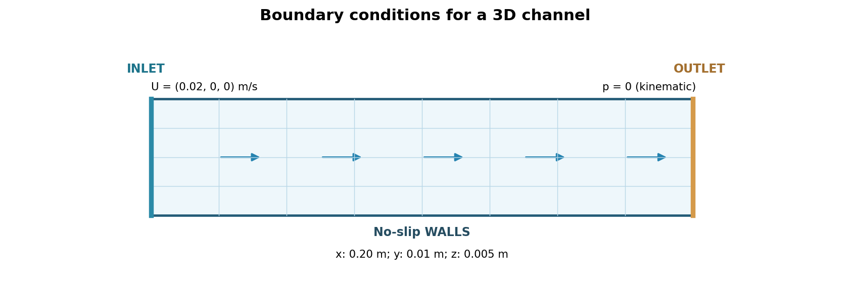
The example models a three-dimensional rectangular duct: length 0.20 m, height 0.010 m, depth 0.005 m. Its 80 × 16 × 8 = 10,240 cells have three boundary patches: inlet, outlet, and walls. The example fluid has ν = 1 × 10⁻⁶ m²/s and the first scenario sets U = (0.020, 0, 0) m/s at the inlet. We use ρ = 1000 kg/m³ only when converting computed kinematic pressure into pascals: the incompressible constant-kinematic-viscosity solver does not require it as an input.
| Quantity | Value | Interpretation |
|---|---|---|
| Inlet area A | 5 × 10⁻⁵ m² | Height × depth |
| Nominal flow Q | 1 × 10⁻⁶ m³/s | Q = A · mean inlet speed |
| Hydraulic diameter Dₕ | 6.667 × 10⁻³ m | Dₕ = 2ab/(a+b) |
| Hydraulic Reynolds number | approximately 133.3 | Re = U Dₕ / ν |
| Convective time L/U | 10 s | A physical time estimate, not steady-state deltaT |
The simple channel deliberately isolates the effects of changes to boundary conditions and viscosity. This is a controlled teaching example, not experimental validation or proof of mesh independence (see Guide 4).
Deep dive · The analytic solution for the rectangular duct: the numbers to expect
For fully developed laminar flow in a rectangular duct there is a series solution (Shah and London). With a 10 mm × 5 mm section (aspect ratio 0.5) the product of Darcy friction factor and Reynolds number is f_D·Re ≈ 62.19 (Fanning 15.55). Hence:
| Quantity | ν = 1·10⁻⁶ m²/s | ν = 2·10⁻⁶ m²/s |
|---|---|---|
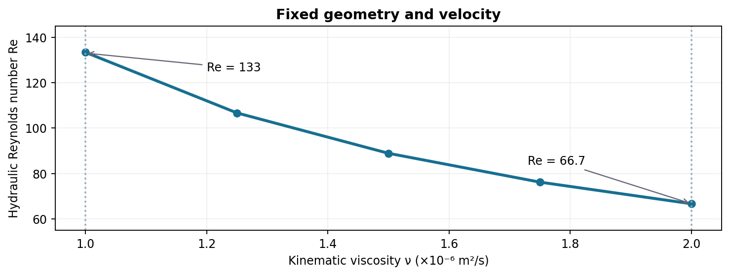
| Re (Dₕ) | 133.3 | 66.7 |
| f_D | 0.466 | 0.933 |
| developed pressure gradient | ≈ 14.0 Pa/m | ≈ 28.0 Pa/m |
| Δp over 0.20 m, developed part only | ≈ 2.80 Pa (2.80·10⁻³ m²/s²) | ≈ 5.60 Pa (5.60·10⁻³ m²/s²) |
| centreline maximum velocity | ≈ 0.0398 m/s (1.99·U) | ≈ 0.0398 m/s |
| entrance length ≈ 0.05·Re·Dₕ | ≈ 44 mm (22 % del canale) | ≈ 22 mm |
With a uniform inlet the computed Δp will be higher than the developed value: the entrance region adds a lumped loss due to core acceleration and higher wall shear. For a clean comparison with theory measure the gradient between two sections in the developed region, for example x = 0.10 m and x = 0.18 m, not between inlet and outlet. This is a genuine verification check, far more informative than a bare “STATUS OK”.
# expected developed gradient and Δp (Python, standard library only)
fRe, Dh, U, nu, rho, L = 62.19, 2*0.01*0.005/0.015, 0.02, 1e-6, 1000, 0.08
Re = U*Dh/nu
dpdx = fRe/Re/Dh * 0.5*rho*U**2          # Pa/m
print(Re, dpdx, dpdx*L, dpdx*L/rho)     # Re, Pa/m, Pa on L, m2/s2 on L
Deep dive · The case mesh and profile resolution
Cells are 2.5 mm in x and 0.625 mm in y and z: aspect ratio 4, aligned with the flow direction, where gradients are weak. There are 8 cells across the short side (5 mm) and 16 across the long side (10 mm): for a nearly parabolic profile this resolves the shape, but a quantitative comparison with the maximum velocity (1.99·U) or the pressure gradient requires the convergence study of Guide 4, for example with 40×8×4, 80×16×8 and 160×32×16 cells (ratio r = 2).
Deep dive · Why this channel cannot be reduced to 2D
The temptation to save cells with a two-dimensional model leads here to gross errors, because the depth (5 mm) is smaller than the height (10 mm) and the side walls dominate friction. Developed pressure gradient at the same mean velocity (0.02 m/s, μ = 10⁻³ Pa·s):
| Model | Formula | Gradient |
|---|---|---|
| 3D rectangular duct | f_D·Re = 62.19 | ≈ 14.0 Pa/m |
| parallel plates, 10 mm gap (2D x–y) | 12·μ·U / h² | 2.4 Pa/m |
| parallel plates, 5 mm gap (2D x–z) | 12·μ·U / h² | 9.6 Pa/m |
A 2D model is legitimate only when the neglected dimension is much larger than the others (section aspect ratio of at least 8–10) or when the problem is truly planar by symmetry. It is a modelling decision to be justified with numbers, not a computational shortcut.
4. Patches: the contract between mesh and fields
The mesh patch inlet in system/blockMeshDict must appear under exactly that name in both 0/U and 0/p; the same applies to outlet and walls. A geometrical patch type (patch, wall, symmetryPlane, etc.) is distinct from the field boundary type (fixedValue, zeroGradient, noSlip, etc.). These are not interchangeable.
| Condition | What it imposes | Common use and limitation |
|---|---|---|
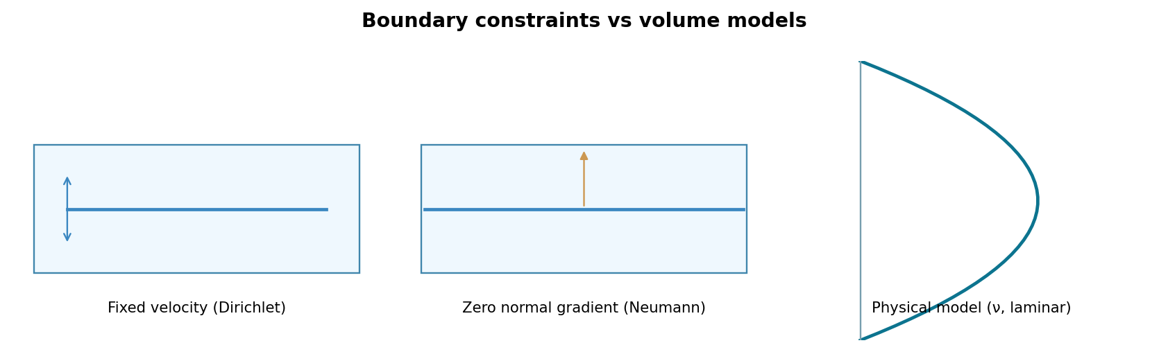
fixedValue | Fixed field value (Dirichlet) | Inlet velocity, pressure reference |
zeroGradient | Zero normal gradient (homogeneous Neumann) | Inlet pressure or simple velocity outlet |
noSlip | Zero velocity on a stationary solid wall | Viscous walls; not equivalent to slip |
flowRateInletVelocity | Prescribed rate with an inferred normal velocity | Useful when Q, rather than U, is known |
pressureInletOutletVelocity | Velocity condition on a pressure-type boundary | Accommodates reverse flow; does not cure a poor outlet placement |
inletOutlet | Outlet condition with a fallback inflow value | Often used for transported scalars; requires inletValue |
symmetryPlane / empty | Special geometric constraints | Must agree with mesh type; empty applies only to genuinely 2D setups |
Warning: zeroGradient does not mean zero pressure or prescribed flow. An outlet placed too close to a wake may affect the solution, whatever boundary formula is chosen; check domain length separately.
Deep dive · Patch type and condition type: which wins and why
The geometric type written in constant/polyMesh/boundary constrains the allowed conditions. empty, symmetryPlane, wedge and cyclic patches are constraint types: the field type must be the same, otherwise the solver stops. The wall type imposes nothing on velocity and pressure fields, but it is required by functions that look for walls: wall distance, RAS wall functions, y⁺ and wallShearStress computation. A wall declared as patch works in laminar flow but silently breaks a turbulent case.
foamDictionary constant/polyMesh/boundary -entry walls/type -value 2>/dev/null || grep -A3 walls constant/polyMesh/boundary
foamDictionary 0/U -entry boundaryField -keywords
foamDictionary 0/p -entry boundaryField -keywords
Deep dive · Inlets and outlets in real situations: the most used conditions
| Situation | U | p | Note |
|---|---|---|---|
| known flow rate | flowRateInletVelocity | zeroGradient | uniform profile or, in recent versions, a profile option |
| measured profile | fixedValue non-uniform or tabulated | zeroGradient | the profile must honour the flow rate |
| reservoir at known pressure | pressureInletOutletVelocity | totalPressure | the flow rate becomes a result |
| outlet with possible backflow | inletOutlet (inletValue (0 0 0)) | fixedValue / totalPressure | prevents backflow from entering with arbitrary velocity |
| moving wall | movingWallVelocity / fixedValue | zeroGradient | lid-driven cavity, belts |
| frictionless wall | slip | zeroGradient | only where friction is truly negligible |
Exact names and required entries of each condition are checked in the API documentation of your version or with foamInfo (Part 8 of the path).
foamInfo flowRateInletVelocity
foamInfo pressureInletOutletVelocity
foamInfo totalPressure
Deep dive · Time-dependent and mixed conditions
For an inlet varying in time (gradual start-up, pulsation) use a condition that reads a function of time, for example an interpolated table; for Robin-type conditions combining value and gradient there is mixed. Example of a 10 s inlet ramp, for transient cases only:
inlet
{
    type            uniformFixedValue;
    uniformValue    table
    (
        (0    (0    0 0))
        (10   (0.02 0 0))
    );
}
The syntax of time functions (table, tableFile, sine, …) is checked with foamInfo uniformFixedValue. In a steady case a ramp has no physical meaning: “time” counts iterations.
Deep dive · Pressure reference without a fixed-pressure patch
If no patch fixes pressure (for example a closed domain, or a duct with both inlet and outlet at fixed velocity), the pressure level is undetermined and must be fixed in one cell. In the algorithm dictionary add pRefCell (or pRefPoint) and pRefValue. In a closed domain the net imposed flow rate must be exactly zero, otherwise the pressure equation has no solution.
PIMPLE
{
    // ...
    pRefPoint   (0.1 0.005 0.0025);
    pRefValue   0;
}
5. Initial and boundary fields: 0/U and 0/p
The supplied velocity file 0/U sets an initially stationary interior and a uniform inlet:
dimensions      [0 1 -1 0 0 0 0];
internalField   uniform (0 0 0);
boundaryField
{
    inlet  { type fixedValue; value uniform (0.02 0 0); }
    outlet { type zeroGradient; }
    walls  { type noSlip; }
}
The file 0/p fixes a kinematic pressure reference at the outlet:
dimensions      [0 2 -2 0 0 0 0];
internalField   uniform 0;
boundaryField
{
    inlet  { type zeroGradient; }
    outlet { type fixedValue; value uniform 0; }
    walls  { type zeroGradient; }
}
Here, the imposed value p=0 defines a pressure reference; it does not mean the liquid’s absolute pressure is zero. For this incompressible formulation, Δp_physical = ρ · Δp_kinematic; the p field is expressed in m²/s², not in pascals.
Background — initial fields. In a steady-state calculation, internalField uniform (0 0 0) is an initial iterate, not necessarily a physical field at time zero. Inadequate initialisation can slow convergence or lead the numerical procedure toward an undesired solution.
Deep dive · The complete case files: 0/U and 0/p
/* OpenFOAM Foundation 14 - Guide 7 (original educational case) */
FoamFile
{
    version 2.0;
    format ascii;
    class volVectorField;
    location "0";
    object U;
}

dimensions      [0 1 -1 0 0 0 0];
internalField   uniform (0 0 0);
boundaryField
{
    inlet
    {
        type fixedValue;
        value uniform (0.02 0 0);
    }
    outlet
    {
        type zeroGradient;
    }
    walls
    {
        type noSlip;
    }
}
/* OpenFOAM Foundation 14 - Guide 7 (original educational case) */
FoamFile
{
version 2.0;
format ascii;
class volScalarField;
location "0";
object p;
}
// Incompressible kinematic pressure: p_phys/rho, in m2/s2.
dimensions [0 2 -2 0 0 0 0];
internalField uniform 0;
boundaryField
{
inlet
{
type zeroGradient;
}
outlet
{
type fixedValue;
value uniform 0;
}
walls
{
type zeroGradient;
}
}Dimensions follow OpenFOAM’s SI order [mass length time temperature amount current luminosity]: [0 1 -1 0 0 0 0] is m/s, [0 2 -2 0 0 0 0] is m²/s². OpenFOAM checks the dimensional consistency of every operation: a pressure written in Pa [1 -1 -2 0 0 0 0] in a kinematic solver produces a dimension error, not a silent wrong result.
Deep dive · Better initialisation: potentialFoam and non-uniform fields
Starting from zero velocity is legitimate but slow: the first iterations must “invent” a field satisfying continuity. Two practical alternatives. The first is to initialise the internal field with the mean velocity, internalField uniform (0.02 0 0);, which already honours the flow rate. The second is to solve a potential flow satisfying ∇·U = 0 with the same boundary conditions and use it as the initial field:
potentialFoam -help
potentialFoam -writep > logs/log.potentialFoam 2>&1   # writes U (and p) into 0/
potentialFoam overwrites the fields in 0/: run it on the working copy, never on the template, and record the fact. In steady cases the final solution must not depend on initialisation; if it does, the problem has multiple solutions or is not converged.
Deep dive · Uniform inlet or developed profile: consequences for the measurements
The template’s uniform inlet is a convenience: it creates a development region of about 44 mm in which pressure gradient and wall stress exceed the developed value. If the goal is the behaviour of the channel within a network, impose the developed profile or extend the domain upstream and measure only downstream. A practical option, in versions that offer it, is the profile parameter of flowRateInletVelocity (laminar or turbulent boundary-layer profiles); in any case the choice must be declared on the case sheet.
6. Material, transport model and numerical method
The material file constant/physicalProperties contains:
viscosityModel constant;
nu             1e-06;
The file constant/momentumTransport contains:
simulationType laminar;In system/controlDict, solver incompressibleFluid; chooses the solver module. In system/fvSchemes, ddtSchemes { default steadyState; } configures steady discretisation. In system/fvSolution, PIMPLE controls pressure-velocity coupling while solvers and relaxationFactors select the linear solvers and numerical relaxation. These represent different design choices: physics, momentum model and numerics.
Why not simply switch to kOmegaSST? A RAS turbulence model requires additional fields (k, omega, nut), consistent inlet turbulence conditions, appropriate wall functions and a near-wall mesh strategy. Changing one line is insufficient. With Re ≈ 133 in this channel, a turbulent model would not be justified solely by the nominal channel dimensions.
Deep dive · The complete constant/ and system/ dictionaries
/* OpenFOAM Foundation 14 - Guide 7 (original educational case) */
FoamFile
{
    version 2.0;
    format ascii;
    class dictionary;
    location "constant";
    object physicalProperties;
}

viscosityModel constant;
nu             1e-06;  // m2/s; example fluid
/* OpenFOAM Foundation 14 - Guide 7 (original educational case) */
FoamFile
{
version 2.0;
format ascii;
class dictionary;
location "constant";
object momentumTransport;
}
simulationType laminar;/* OpenFOAM Foundation 14 - Guide 7 (original educational case) */
FoamFile
{
version 2.0;
format ascii;
class dictionary;
location "system";
object controlDict;
}
solver incompressibleFluid;
startFrom startTime;
startTime 0;
stopAt endTime;
endTime 700;
deltaT 1; // pseudo-time iteration for steadyState
writeControl timeStep;
writeInterval 100;
purgeWrite 0;
writeFormat ascii;
writePrecision 9;
writeCompression off;
timeFormat general;
timePrecision 6;
runTimeModifiable true;
functions
{
inletFlux
{
type surfaceFieldValue;
libs ("libfieldFunctionObjects.so");
log true;
writeControl writeTime;
writeFields false;
patch inlet;
operation sum;
fields (phi);
}
outletFlux
{
type surfaceFieldValue;
libs ("libfieldFunctionObjects.so");
log true;
writeControl writeTime;
writeFields false;
patch outlet;
operation sum;
fields (phi);
}
}/* OpenFOAM Foundation 14 - Guide 7 (original educational case) */
FoamFile
{
version 2.0;
format ascii;
class dictionary;
location "system";
object fvSchemes;
}
ddtSchemes
{
default steadyState;
}
gradSchemes
{
default Gauss linear;
}
divSchemes
{
default none;
div(phi,U) bounded Gauss linearUpwind grad(U);
div((nuEff*dev2(T(grad(U))))) Gauss linear;
}
laplacianSchemes
{
default Gauss linear corrected;
}
interpolationSchemes
{
default linear;
}
snGradSchemes
{
default corrected;
}
wallDist
{
method meshWave;
}/* OpenFOAM Foundation 14 - Guide 7 (original educational case) */
FoamFile
{
version 2.0;
format ascii;
class dictionary;
location "system";
object fvSolution;
}
solvers
{
p
{
solver GAMG;
smoother DIC;
tolerance 1e-8;
relTol 0.05;
}
pFinal
{
$p;
relTol 0;
}
U
{
solver smoothSolver;
smoother symGaussSeidel;
tolerance 1e-10;
relTol 0.1;
}
UFinal
{
$U;
relTol 0;
}
}
PIMPLE
{
momentumPredictor no;
nOuterCorrectors 1;
nNonOrthogonalCorrectors 0;
}
relaxationFactors
{
fields { p 0.3; }
equations { U 0.7; }
}/* OpenFOAM Foundation 14 - Guide 7 (original educational case) */
FoamFile
{
version 2.0;
format ascii;
class dictionary;
location "system";
object blockMeshDict;
}
scale 1;
vertices
(
(0 0 0) (0.20 0 0) (0.20 0.01 0) (0 0.01 0)
(0 0 0.005) (0.20 0 0.005) (0.20 0.01 0.005) (0 0.01 0.005)
);
blocks ( hex (0 1 2 3 4 5 6 7) (80 16 8) simpleGrading (1 1 1) );
edges ();
boundary
(
inlet
{
type patch;
faces ((0 4 7 3));
}
outlet
{
type patch;
faces ((1 2 6 5));
}
walls
{
type wall;
faces ((0 1 5 4) (3 7 6 2) (0 3 2 1) (4 5 6 7));
}
);
mergePatchPairs ();Deep dive · The case fvSchemes and fvSolution, entry by entry
| Entry | Choice | Engineering rationale |
|---|---|---|
ddtSchemes | steadyState | no time term: “Time” counts iterations |
div(phi,U) | bounded Gauss linearUpwind grad(U) | second-order upwind; bounded removes the non-zero ∇·U part during convergence, typical for steady runs |
laplacianSchemes | Gauss linear corrected | orthogonal mesh: non-orthogonal correction inactive but ready |
wallDist meshWave | — | unused in laminar flow; needed by RAS models |
p: GAMG + DIC | tolerance 1e-8, relTol 0.05 | multigrid for the elliptic pressure equation |
U: smoothSolver symGaussSeidel | relTol 0.1 | diagonally dominant equation, a simple solver suffices |
pFinal / UFinal | relTol 0 | settings of the last correction of the PIMPLE loop |
momentumPredictor no | — | reduces cost per iteration at low Reynolds number |
relaxationFactors | p 0.3, U 0.7 | classic SIMPLE values for stability |
Parts 5 and 6 of the path explain schemes and solvers in detail. To know which entries your installation uses in steady cases, compare with the pitzDailySteady tutorial: it is the safest reference for version-14 keywords.
Deep dive · What it would really take to switch to a RAS model
constant/momentumTransport:simulationType RAS;and a sub-dictionaryRAS { model kOmegaSST; turbulence on; printCoeffs on; }.- New fields
0/k,0/omega,0/nut, with consistent inlet conditions and wall functions (kqRWallFunction,omegaWallFunction,nutkWallFunctionor low-Reynolds equivalents). - Schemes for
div(phi,k)anddiv(phi,omega), solvers and relaxation forkandomega. - A wall mesh consistent with the chosen treatment (Guide 6, y⁺).
Typical inlet values: k = 1.5·(I·U)² with intensity I of a few percent and ω = √k / (C_μ^¼·ℓ) with C_μ = 0.09 and a length scale ℓ linked to the hydraulic diameter (for example 0.07·Dₕ). At Re ≈ 133 none of this is justified: a turbulence model in a laminar flow adds spurious viscosity and corrupts Δp. The correct starting point, when needed, is your installation’s RAS tutorial.
Deep dive · Non-Newtonian viscosity: where it is set and how to check it
With fluids such as blood, polymers or slurries the viscosity depends on the strain rate. In Foundation 14 the model is selected in constant/physicalProperties with viscosityModel; available names and required coefficients come from the installed tutorials, not from examples for other versions:
grep -rh --include=physicalProperties "viscosityModel" "$FOAM_TUTORIALS" | sort | uniq -c
grep -rl --include=physicalProperties -E "CrossPowerLaw|BirdCarreau|powerLaw|HerschelBulkley" "$FOAM_TUTORIALS" | head
With variable viscosity this guide’s analytic solution no longer holds, the profile flattens (shear-thinning fluids) and the Reynolds number must be defined with a declared reference viscosity. This step comes after the Newtonian case has been verified.
Deep dive · Relaxation and algorithm: convergence speed versus stability
With the classic factors p 0.3 and U 0.7 the SIMPLE algorithm converges robustly but slowly. The “consistent” variant (SIMPLEC), where available, allows higher factors (for example U 0.9 and no pressure relaxation) and considerably reduces the iteration count. The criterion for changing is empirical but measurable: compare the iterations needed to bring residuals below threshold and check that the final solution (Δp, Q) does not change. Version-14 keywords are checked in pitzDailySteady.
7. Working from Windows
The package layout is:
examples/channel_case/           # complete original template
examples/alternatives/           # flow-rate BC, alternative viscosity
scripts/run_case.sh              # creates unique copies and runs OpenFOAM
scripts/preflight.py             # optional static structural test
figures/                         # illustrations
results/                         # generated by the run script
Extract the package on Windows, edit plain-text configuration with Notepad++ while preserving UTF-8 and Unix LF line endings, and transfer the complete directory with FileZilla over SFTP. Open PowerShell and connect:
ssh user@server.exampleFrom the directory containing examples/ and scripts/ on Linux:
source /opt/OpenFOAM-14/etc/bashrc
foamVersion
chmod +x scripts/run_case.sh
./scripts/run_case.sh velocity
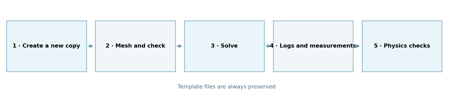
The launcher determines its own directory and creates a unique results/velocity_..._XXXXXX working directory. No existing template or previous run is overwritten. For long calculations use tmux (Guide 1).
Deep dive · The complete run_case.sh script
#!/usr/bin/env bash
# GNU GPL v3 or later - Guide 7. Never changes the shipped template.
set -Eeuo pipefail
ROOT="$(cd "$(dirname "${BASH_SOURCE[0]}")/.." && pwd)"
TEMPLATE="$ROOT/examples/channel_case"
OUTPUT="$ROOT/results"
MODE="${1:-}"
case "$MODE" in
  velocity|flowrate|viscosity) ;;
  *) echo "Usage: $0 velocity|flowrate|viscosity" >&2; exit 2;;
esac
for executable in blockMesh checkMesh foamRun; do
  command -v "$executable" >/dev/null 2>&1 || { echo "Missing $executable: source OpenFOAM-14/etc/bashrc" >&2; exit 127; }
done
mkdir -p "$OUTPUT"
DEST="$(mktemp -d "$OUTPUT/${MODE}_$(date -u +%Y%m%dT%H%M%SZ)_XXXXXX")"
cp -a "$TEMPLATE/." "$DEST/"
mkdir -p "$DEST/logs"
if [[ "$MODE" == flowrate ]]; then
  cp "$ROOT/examples/alternatives/U_flowrate" "$DEST/0/U"
elif [[ "$MODE" == viscosity ]]; then
  cp "$ROOT/examples/alternatives/physicalProperties_high_nu" "$DEST/constant/physicalProperties"
fi
printf '%s\n' "Mode: $MODE" "Case: $DEST" "UTC: $(date -u +%Y-%m-%dT%H:%M:%SZ)" >"$DEST/logs/RUN_INFO.txt"
CURRENT_STEP=initialisation
onexit() {
  status=$?
  if (( status == 0 )); then
    printf 'OK\n' >"$DEST/logs/STATUS.txt"
  else
    printf 'FAILED during %s (exit code %s)\n' "$CURRENT_STEP" "$status" >"$DEST/logs/STATUS.txt"
  fi
}
trap onexit EXIT
CURRENT_STEP=blockMesh
blockMesh -case "$DEST" >"$DEST/logs/log.blockMesh" 2>&1
CURRENT_STEP=checkMesh
checkMesh -case "$DEST" -allGeometry -allTopology >"$DEST/logs/log.checkMesh" 2>&1
CURRENT_STEP=foamRun
foamRun -case "$DEST" >"$DEST/logs/log.foamRun" 2>&1
printf 'Completed in %s\n' "$DEST"
mktemp -d … _XXXXXXcreates a directory with a random suffix: two launches in the same second never collide.- The
trap onexit EXITwritesSTATUS.txtin every case, even whenset -estops the script: the file says at which stage and with which code it stopped. - Variants are obtained by replacing a single file in the copy (
0/Uorconstant/physicalProperties): the template is never touched. - Exit codes: 2 for an unknown mode, 127 if an OpenFOAM executable is missing; otherwise the failed utility’s code, reported in
STATUS.txt.
Deep dive · The preflight.py static check
#!/usr/bin/env python3
# GNU GPL v3 or later - static structural checks, no OpenFOAM runtime required.
from pathlib import Path
import re, sys
BASE = Path(__file__).resolve().parents[1]
CASE = BASE/'examples/channel_case'
check = [('0/U','volVectorField','U'),('0/p','volScalarField','p'),('constant/physicalProperties','dictionary','physicalProperties'),('constant/momentumTransport','dictionary','momentumTransport'),('system/blockMeshDict','dictionary','blockMeshDict'),('system/controlDict','dictionary','controlDict'),('system/fvSchemes','dictionary','fvSchemes'),('system/fvSolution','dictionary','fvSolution')]
for relative,kind,name in check:
    s=(CASE/relative).read_text()
    assert re.search(r'\bclass\s+'+kind+r'\s*;',s),relative
    assert re.search(r'\bobject\s+'+name+r'\s*;',s),relative
    assert s.count('{') == s.count('}'),relative
    assert s.count('(') == s.count(')'),relative
for fname in ('0/U','0/p'):
    s=(CASE/fname).read_text()
    for patch in ('inlet','outlet','walls'):
        assert re.search(r'\b'+patch+r'\s*\{',s),f'{fname} missing patch {patch}'
u=(CASE/'0/U').read_text()
p=(CASE/'0/p').read_text()
assert 'dimensions      [0 1 -1 0 0 0 0]' in u
assert 'dimensions      [0 2 -2 0 0 0 0]' in p
assert 'solver           incompressibleFluid' in (CASE/'system/controlDict').read_text()
A=.01*.005; U=.02; nu=1e-6; D=2*.01*.005/(.01+.005)
print(f'PASS: 8 dictionaries; patches match; 80*16*8=10240 cells; A={A:.8g} m2; Q={A*U:.8g} m3/s; Re_Dh={U*D/nu:.2f}')
print('WARNING: static check only; does not run blockMesh/checkMesh/foamRun.')
It also runs on Windows, before the transfer: it checks class and name of each dictionary, bracket balance, presence of the three patches in the fields, the dimensions of U and p and the selected solver, and prints reference values (area, flow rate, Reynolds). It does not replace execution: a syntactically correct dictionary can be physically wrong.
python scripts/preflight.pyDeep dive · Running the three variants in sequence, unattended
The three exercises are independent and short: they can be launched in sequence in a tmux session, with a final summary. Each variant creates its own directory, so one failure does not stop the others if set -e is avoided in the loop:
tmux new -s guide7
for m in velocity flowrate viscosity; do ./scripts/run_case.sh "$m" || echo "$m failed"; done
for d in results/*/; do printf '%s %s\n' "$d" "$(cat "$d/logs/STATUS.txt")"; done
python3 scripts/collect_fluxes.py results > flux_summary.csv
8. Three exercises: change one parameter at a time
Exercise A — fixed inlet velocity. Run ./scripts/run_case.sh velocity. It copies the template, executes blockMesh, runs checkMesh -allGeometry -allTopology, and starts foamRun. A new directory contains logs/log.blockMesh, logs/log.checkMesh, logs/log.foamRun, logs/STATUS.txt and logs/RUN_INFO.txt.
Exercise B — prescribed volumetric flow rate. Run ./scripts/run_case.sh flowrate. In the copied 0/U, the inlet is replaced by:
inlet
{
    type flowRateInletVelocity;
    volumetricFlowRate 1e-06;
}
With A = 5×10⁻⁵ m², this corresponds to 0.02 m/s mean inlet speed. The local profile need not be identical in every flow setup, but the pair tests two equivalent ways to specify the same nominal inlet. In flowRateInletVelocity, the positive 1e-06 denotes flow into the domain.
Exercise C — twice the kinematic viscosity. Run ./scripts/run_case.sh viscosity. The copied constant/physicalProperties changes ν to 2×10⁻⁶ m²/s, leaving the fixed inlet unchanged. The hydraulic Reynolds number drops to about 66.7. The pressure loss can increase; precise proportionality with viscosity presumes fully developed laminar conditions, not every inlet development region.
Deep dive · The two package variants, complete
/* OpenFOAM Foundation 14 - Guide 7 (original educational case) */
FoamFile
{
    version 2.0;
    format ascii;
    class volVectorField;
    location "0";
    object U;
}

dimensions      [0 1 -1 0 0 0 0];
internalField   uniform (0 0 0);
boundaryField
{
    inlet
    {
        type flowRateInletVelocity;
        volumetricFlowRate 1e-06; // m3/s (positive into domain)
    }
    outlet { type zeroGradient; }
    walls  { type noSlip; }
}
/* OpenFOAM Foundation 14 - Guide 7 (original educational case) */
FoamFile
{
version 2.0;
format ascii;
class dictionary;
location "constant";
object physicalProperties;
}
viscosityModel constant;
nu 2e-06; // m2/sWith flowRateInletVelocity and a uniform profile the imposed velocity is Q/A = 1·10⁻⁶ / 5·10⁻⁵ = 0.02 m/s: identical to exercise A. The A–B comparison is therefore a consistency test: the two solutions must coincide within solver tolerance. A noticeable difference points to an area, sign or unit error.
Deep dive · What must change between A and C, in numbers
Doubling ν at fixed velocity, in the developed region the pressure gradient doubles (about 14 → 28 Pa/m), because f_D = 62.19/Re and Re halves; the entrance length halves (44 → 22 mm); the developed profile and hence the maximum velocity stay the same, because in laminar flow the profile shape does not depend on ν. The total inlet–outlet Δp grows less than proportionally, because the entrance contribution grows less than the viscous part.
If the run shows a 2.00 ratio between gradients measured in the developed region, the case is verified; if it shows a ratio of 2 on the total Δp, you are probably comparing different quantities or the solution is not converged.
Deep dive · Two more exercises to complete the study
- D — Outlet position. Extend the channel to 0.30 m (vertices and x cell count in proportion, 120 × 16 × 8) keeping everything else: the gradient measured between 0.10 and 0.18 m must not change. If it does, the outlet was affecting the solution.
- E — Refinement. Repeat A with 40 × 8 × 4 and 160 × 32 × 16 cells (r = 2) and apply the Guide 4 procedure to the developed pressure gradient. Compare the extrapolated value with 14.0 Pa/m: a complete verification, numerical and analytic together. The finest mesh has 81,920 cells, still light.
9. Run checks, fluxes and conservation
The numerical outcome must be assessed from logs: STATUS.txt = OK means only that the process completed without reporting a command failure; it does not prove scientific convergence. Inspect FOAM FATAL ERROR, final residuals, continuity errors and the stability of physical observables. The two function objects inletFlux and outletFlux use surfaceFieldValue to sum phi on each patch, following the domain-outward normal convention:
Q_inlet  < 0    # inlet points inward; outward surface normal gives negative flux
Q_outlet > 0    # outlet flow has positive outward flux
Q_inlet + Q_outlet ≈ 0  # volumetric mass-balance consistency
In this incompressible solver, phi is a volumetric flux (m³/s). The example writes values at field-write intervals. Evaluate a relative conservation mismatch such as |Qin + Qout| / max(|Qin|, |Qout|) without treating any arbitrary tolerance as universal. For a pressure-drop study, area-average p on selected sections in ParaView (Guide 3), then multiply the kinematic pressure difference by the selected density to express it in Pa.
Background — conservation versus convergence. Low residuals do not guarantee correct conservation or sensible physical boundary constraints. Conversely, a small inlet–outlet flow mismatch alone does not certify an accurate velocity field. Both types of checks matter.
Deep dive · Convergence of a steady case: automatic criteria and quantity monitoring
The case runs 700 iterations without a stop criterion. In serious use a residual control is added, so the run stops when the initial residuals of all equations fall below declared thresholds. In version 14 the entry goes into the algorithm dictionary; check the exact syntax in the pitzDailySteady tutorial:
grep -n -A6 residualControl "$FOAM_TUTORIALS/incompressibleFluid/pitzDailySteady/system/fvSolution"Residuals alone are not enough: the history of the quantities of interest goes alongside. Here the natural choice is to add mean-pressure measurements on two sections in the developed region and check that their difference stays constant over the last few hundred iterations. An example function object to add to functions in the working copy:
pSections
{
    type            surfaces;
    libs            ("libsampling.so");
    writeControl    writeTime;
    surfaceFormat   raw;
    fields          (p U);
    interpolationScheme cellPoint;
    surfaces
    {
        x010 { type cuttingPlane; point (0.10 0 0); normal (1 0 0); interpolate true; }
        x018 { type cuttingPlane; point (0.18 0 0); normal (1 0 0); interpolate true; }
    }
}
Sampling-surface keywords have changed between versions: before using it compare with foamInfo surfaces or the files in $FOAM_ETC/caseDicts/functions. Alternatively, section averages are computed in ParaView (Guide 3).
Deep dive · Continuity error in the log: how to read it
At every iteration the log prints a “time step continuity errors” line with three numbers: mean local error (sum local), global and cumulative. They are normalised errors on flux divergence after the pressure correction: they must become very small and the “global” one must oscillate around zero without drift. A drifting cumulative value indicates systematic mass loss, typically from too loose pressure tolerances.
grep "continuity errors" logs/log.foamRun | tail -n 3
grep -E "^Time =|Solving for (Ux|p)" logs/log.foamRun | tail -n 8
Deep dive · Comparing the velocity profile with the exact solution
In ParaView, Plot Over Line from (0.15, 0, 0.0025) to (0.15, 0.01, 0.0025) samples the profile across the height at mid-depth, in the developed region. The following script (standard library only) computes the series solution at the same 21 points; the RMSE between the two profiles, normalised by U, measures the local discretisation error (Guide 3).
#!/usr/bin/env python3
"""Analytic fully developed laminar profile in a rectangular duct (series solution).
Prints u/U_mean along the 10 mm side at mid-depth, to compare with a ParaView Plot Over Line CSV."""
import math
H, W, U = 0.010, 0.005, 0.02          # duct height (y), depth (z), mean velocity
a, b = W / 2, H / 2                   # half-widths: a short side, b long side
s = sum(math.tanh((2*k+1)*math.pi*b/(2*a)) / (2*k+1)**5 for k in range(200))
fac = 1 - 192*a/(math.pi**5*b)*s
G = 3*U/(a*a*fac)                      # (-dp/dx)/mu, from the mean velocity

def u(yy, zz, N=60):                  # yy across the short side, zz across the long side
    out = 0.0
    for k in range(N):
        n = 2*k + 1
        arg = n*math.pi*b/(2*a)
        r = math.cosh(n*math.pi*zz/(2*a))/math.cosh(arg) if arg < 700 else math.exp(n*math.pi*(abs(zz)-b)/(2*a))
        out += (-1)**k * (1 - r) * math.cos(n*math.pi*yy/(2*a)) / n**3
    return 16*a*a/math.pi**3 * G * out

print("y_m,u_over_Umean")
for i in range(21):
    y = H*i/20                        # 0 ... 10 mm, wall to wall
print(f"{y:.4f},{u(0.0, y - b)/U:.4f}")| y [mm] | 0 | 1 | 2 | 3 | 4 | 5 | 6 | 7 | 8 | 9 | 10 |
|---|---|---|---|---|---|---|---|---|---|---|---|
| u/U | 0 | 0.99 | 1.53 | 1.82 | 1.95 | 1.99 | 1.95 | 1.82 | 1.53 | 0.99 | 0 |
The profile along the long side is flatter at the centre than a parabola, because at mid-depth the gradient is dominated by the nearby walls (short side). A Poiseuille parabola between parallel plates would give a maximum of 1.5·U: a result close to 1.5 would indicate a geometry error or an unintentionally two-dimensional case.
10. Common faults and targeted diagnosis
| Symptom | Suspected cause | Specific check |
|---|---|---|
| Missing patch | Name mismatch between mesh, 0/U or 0/p | Compare constant/polyMesh/boundary with fields |
physicalProperties error | Mixing different OpenFOAM releases | Compare with $FOAM_TUTORIALS/incompressibleFluid/cylinder |
| Pressure dimension error | Confusing Pa with kinematic pressure | Expected [0 2 -2 0 0 0 0] |
| Divergence | Inconsistent inlet, poor mesh, aggressive scheme | Read the first error, rerun checkMesh, simplify |
| Inlet/outlet imbalance | Unconverged solution or reverse flow | Check face-normal signs and iteration history |
RAS model missing k, omega | Enabling a model without its fields | Start from a valid RAS tutorial and verify wall conditions |
| Unexpected pressure drop | Geometry, inlet development, units or wrong probes | Check dimensions, density and section placement |
Altering a boundary condition changes the physical question. Always log and compare that change in a separate case copy, never silently modify a published result.
Deep dive · Reading the first error: anatomy of a FOAM FATAL ERROR
A fatal error reports the message, the file and often the line of the dictionary involved, and the code function that raised it. The useful message is the one before “From function”; the stack lines that follow are for developers. The most frequent errors at this stage: “Cannot find patchField entry for walls” (different patch name), “keyword nu is undefined” (dictionary from another release), “Different dimensions for (p + …)” (wrong units), “Unknown patchField type” (misspelt condition or not available in the version).
grep -n -m1 -B2 -A12 "FOAM FATAL" logs/log.foamRun
cat logs/STATUS.txt
Deep dive · Divergence in the first iterations: a four-step procedure
- Read in which equation the residual blows up first (
Uxorp) and at which iteration. - Re-run
checkMeshand compare with Guide 6: a freshly modified mesh is the first suspect. - Reduce relaxation factors (for example
p 0.2,U 0.5) and temporarily switch tobounded Gauss upwindfordiv(phi,U): if it then converges, the problem is numerical; if it still diverges, it is in the boundary conditions. - Restore the original settings starting from the converged solution (
startFrom latestTime): the second-order scheme must be the one used for the final result.
11. What to retain as scientific evidence
For each variant, archive 0/, constant/, system/, solver/version, logs/, cell count, inlet/outlet fluxes, pressure difference, unit conventions, convergence criteria and the ParaView .pvsm state if used. FileZilla can download small logs and CSVs for Windows-based analysis; there is usually no reason to transfer every large flow-field file if pvserver can read them on Linux.
Final checklist
- ☐ I have confirmed Foundation 14 and the
incompressibleFluidmodule. - ☐ Every mesh patch matches its field configuration.
- ☐ I have checked area, units and nominal flow rate.
- ☐ The original templates remain unchanged.
- ☐ Meshing, mesh validation and solution ran in an identifiable new case.
- ☐ I have inspected convergence, conservation and physical observables.
- ☐ I have distinguished kinematic pressure from pressure in pascals.
- ☐ I have recorded exactly which setting differs across the three cases.
Deep dive · A ready-to-fill case sheet
| Field | Exercise A (design values) |
|---|---|
| version and solver | OpenFOAM Foundation 14, foamRun / incompressibleFluid |
| mesh | 80×16×8 = 10,240 cells, checkMesh OK |
| fluid | ν = 1e-6 m²/s; ρ = 1000 kg/m³ (post-processing only) |
| inlet | fixedValue U = 0.02 m/s, Q = 1e-6 m³/s |
| outlet / walls | p = 0 (fixedValue) / noSlip |
| numerics | steadyState, linearUpwind, PIMPLE, p 0.3 / U 0.7 |
| stop criterion | 700 iterations (to be replaced by residualControl) |
| Q_in, Q_out, imbalance | from collect_fluxes.py |
| p gradient in developed region | expected ≈ 1.40e-2 m²/s² per m (14 Pa/m) |
Deep dive · A fingerprinted delivery archive
The same scheme as Guide 5 applies here: one archive per variant, without the intermediate fields that can be regenerated, with file fingerprints and an environment description.
for d in results/*/; do
  ( cd "$d" && { date -u; foamVersion; } > logs/environment.txt 2>&1
    find 0 constant system logs postProcessing -type f -print0 | sort -z | xargs -0 sha256sum > logs/files.sha256 )
  tar czf "$(basename "$d").tar.gz" -C "$d" 0 constant/physicalProperties constant/momentumTransport system logs postProcessing
done
12. Operational appendix: patch measurements and comparison criteria
The function objects are defined in the functions section of system/controlDict. The supplied case already includes inletFlux and outletFlux, each summing phi over a selected mesh patch. For example, the actual inlet measurement block is:
inletFlux
{
    type surfaceFieldValue;
    libs ("libfieldFunctionObjects.so");
    log true;
    writeControl writeTime;
    writeFields false;
    patch inlet;
    operation sum;
    fields (phi);
}
A typical postProcessing/inletFlux/0/surfaceFieldValue.dat file stores a numerical time marker and a flux value on each data line. A corresponding outlet file is written under postProcessing/outletFlux/.... Do not compare an early inlet line with a late outlet line: measurements must refer to the same calculation state. The provided portable Python script scripts/collect_fluxes.py selects the latest available value for both objects in each run directory and generates a CSV. Missing data remain empty: values are never made up. You may download only logs/ and postProcessing/ with FileZilla, provided the nested directory layout is preserved.
python scripts/collect_fluxes.py results > flux_summary.csvWorked measurement reasoning. An imposed flow of 1×10⁻⁶ m³/s is 1 mL/s. For the specified orientation, a physically consistent result should have approximately −1×10⁻⁶ m³/s through the inlet and +1×10⁻⁶ m³/s through the outlet. Do not imply more significant digits than the discretisation and solver justify. Compare pressure on defined physical sections, rather than arbitrarily chosen cells.
A common experimental-design error: change inlet flow, viscosity, mesh and outlet position all at once, then attribute the change in ΔP to a single cause. The three separate runs instead isolate one change at a time. For quantitative work, also check mesh independence, inlet-development effects and numerical sensitivity.
Background — iterative time. When ddtSchemes is set to steadyState, deltaT 1 and the printed Time values essentially index pseudo-time/iterations. A trend against this index is not a physical transient response. True unsteady analysis requires different temporal schemes, numerical controls, time-step verification and a Courant-number assessment.
Deep dive · The complete collect_fluxes.py script
#!/usr/bin/env python3
# GPL-3.0-or-later. Parse OpenFOAM 14 surfaceFieldValue output on Linux or Windows.
"""Usage: python scripts/collect_fluxes.py results > flux_summary.csv
Read last numeric time row from postProcessing/{inletFlux,outletFlux}/*/surfaceFieldValue.dat.
Missing values remain blank; script never fabricates simulation outputs.
"""
from pathlib import Path
from csv import writer
from sys import argv, stdout, stderr
from math import isfinite

def read_series(case, name):
    rows={}
    for f in (case/'postProcessing'/name).glob('*/surfaceFieldValue.dat'):
        with f.open(encoding='utf-8',errors='replace') as inp:
            for line in inp:
                if not line.strip() or line.lstrip().startswith('#'):
                    continue
                parts=line.split()
                if len(parts)<2:continue
                try: x=float(parts[0]);y=float(parts[1])
                except ValueError:continue
                if isfinite(x) and isfinite(y):
                    old=rows.get(x)
                    if old is None or f.stat().st_mtime >= old[0]:
                        rows[x]=(f.stat().st_mtime,y)
    return {t:value for t,(_,value) in rows.items()}

def main():
    if len(argv)!=2:
        print('usage: collect_fluxes.py <results-directory>',file=stderr);return 2
    root=Path(argv[1]);
    if not root.is_dir():
        print(f'not a directory: {root}',file=stderr);return 2
    cw=writer(stdout,lineterminator='\n')
    cw.writerow(['case','status','Q_inlet_m3s','Q_outlet_m3s','imbalance_relative'])
    for case in sorted(p for p in root.iterdir() if p.is_dir()):
        status_file=case/'logs'/'STATUS.txt'
        status=status_file.read_text(encoding='utf-8').strip() if status_file.exists() else 'UNKNOWN'
        ins=read_series(case,'inletFlux');outs=read_series(case,'outletFlux')
        common=ins.keys() & outs.keys()
        t=max(common) if common else None
        qi=ins.get(t);qo=outs.get(t)
        imb=abs(qi+qo)/max(abs(qi),abs(qo)) if qi is not None and qo is not None and max(abs(qi),abs(qo))>0 else None
        cw.writerow([case.name,status,qi if qi is not None else '',qo if qo is not None else '',imb if imb is not None else ''])
    return 0
if __name__=='__main__':raise SystemExit(main())- It keeps one value per time; if the same time appears in several files (restarts), the most recently modified file wins.
- It uses the last time common to both measurements, so it never compares different times.
- The imbalance is relative:
|Qin + Qout| / max(|Qin|, |Qout|); if a value is missing the cell stays empty.
With the nominal case one expects Q_in ≈ −1·10⁻⁶ and Q_out ≈ +1·10⁻⁶ m³/s; the relative imbalance of a converged incompressible case is of the order of the pressure tolerance, well below 10⁻⁶.
Deep dive · Also measuring wall shear stress and comparing it with Δp
In the developed region the force balance on a volume of length L gives Δp·A = τ̄_w·P·L, with P the wetted perimeter (30 mm). It is a second independent check: with 14 Pa/m and A/P = Dₕ/4 = 1.667 mm the expected mean wall stress is τ̄_w ≈ 0.023 Pa. In OpenFOAM wall shear stress is computed with the wallShearStress function object (kinematic, multiply by ρ) and averaged over the patch in ParaView or with surfaceFieldValue.
foamPostProcess -help
foamPostProcess -func wallShearStress -latestTime   # on the working copy, after the run
13. Repeating measurements and building a credible comparison
For every run, retrieve at least logs/, postProcessing/, 0/, constant/ and system/ via FileZilla. Import the CSVs into your Windows analysis tool, label every column with its units, and record imposed speed/rate, ν, Re, measured flux, conservation mismatch, and ΔP when available. Do not draw a pressure-loss comparison until the measurement sections and averaging procedures are consistent across cases.
| Comparison | Held constant | Changed variable | Interpretation to check |
|---|---|---|---|
| A versus B | Nominal Q, ν and mesh | fixedValue versus flowRateInletVelocity | Practical equivalence despite inlet-profile development |
| A versus C | Geometry, imposed inlet U, mesh | ν from 1×10⁻⁶ to 2×10⁻⁶ | Reynolds number and viscous resistance change |
| All three | Patch names and solver | Only the declared parameter | Conservation, residuals and observable stability |
Verification does not end when the script reports OK. Review the results independently: look for unexplained systematic changes, compare mean speeds and pressure gradients, assess entrance and outlet effects and plan mesh refinement. Each refined mesh must be saved as a new case, and the comparison extended according to Guide 4.
Deep dive · How small the difference between A and B must be
A and B impose the same inlet field, so the difference between their solutions measures only iterative noise. A reasonable engineering criterion: the difference in the quantities of interest (Δp between the two sections, Q) must be at least an order of magnitude smaller than any effect you want to attribute to physics, for example the A–C difference. If A and B differ by more than 1 %, iterative convergence is insufficient and the A–C comparison is not yet interpretable.
Deep dive · The comparison sheet: columns and units
case,inlet_bc,nu_m2_s,Re_Dh,Q_in_m3_s,Q_out_m3_s,imbalance_rel,dpdx_developed_Pa_m,dp_total_Pa,umax_m_s,iterations,notes
A_velocity,fixedValue 0.02,1e-6,133.3,,,,,,,,
B_flowrate,flowRateInletVelocity 1e-6,1e-6,133.3,,,,,,,,
C_viscosity,fixedValue 0.02,2e-6,66.7,,,,,,,,
Expected values for verification: dpdx_developed ≈ 14.0 / 14.0 / 28.0 Pa/m; umax ≈ 0.0398 m/s in all three cases. Empty columns are filled with data from collect_fluxes.py and ParaView; units are in the column name, so the file stays readable out of context.
14. Official sources and verification limits
- OpenFOAM Foundation 14 tutorial source: https://github.com/OpenFOAM/OpenFOAM-14/tree/master/tutorials/incompressibleFluid/cylinder
- OpenFOAM 14
incompressibleFluidsource: https://github.com/OpenFOAM/OpenFOAM-14/blob/master/applications/modules/incompressibleFluid/incompressibleFluid.C - Foundation 14 API,
flowRateInletVelocity: https://cpp.openfoam.org/v14/classFoam_1_1flowRateInletVelocityFvPatchVectorField.html - Foundation 14 API,
surfaceFieldValue: https://cpp.openfoam.org/v14/classFoam_1_1functionObjects_1_1fieldValues_1_1surfaceFieldValue.html - Foundation 14 API,
pressureInletOutletVelocity: https://cpp.openfoam.org/v14/classFoam_1_1pressureInletOutletVelocityFvPatchVectorField.html
Verification status: exercise files have passed static checks for structure, patch names, scripts, units and hand-calculated reference quantities. First execution on a Linux server should be treated as an acceptance test; use Guides 2–4 for numerical and physical verification.
Deep dive · Reading for the next step
- R. K. Shah, A. L. London, Laminar Flow Forced Convection in Ducts, Academic Press, 1978. Solutions and correlations for ducts of any section, including f·Re for rectangles.
- F. M. White, Viscous Fluid Flow, McGraw-Hill. Laminar duct flow, entrance length, boundary layer.
- S. B. Pope, Turbulent Flows, Cambridge University Press, 2000. Foundations of the RAS and LES models mentioned in section 6.
- Tutorials in your installation:
incompressibleFluid/pitzDailySteady,incompressibleFluid/cylinder, to compare entry by entry with the guide’s case.
Related guides: Linux server from Windows, monitoring and convergence, ParaView for quantitative analysis, verification and validation, parameter sweeps, mesh generation and quality checks and the Learning OpenFOAM 14 path.