

OpenFOAM: mesh generation and quality checks with blockMesh and snappyHexMesh
Sixth operating guide on OpenFOAM installed on a Linux server and used from Windows, after those on server and transfers, monitoring and convergence, quantitative analysis with ParaView, verification and validation and parameter sweeps. This one goes upstream of the run: mesh generation and quality checks with blockMesh and snappyHexMesh. The deep-dive boxes open with a click: they contain the complete package files, the expected numbers to check every step, and additional procedures.
From CAD geometry to blockMesh and snappyHexMesh
Practical handbook for OpenFOAM Foundation 14 · Windows workstation · Linux computation server
Edition: October 2026 · Scope: preprocessing and mesh diagnostics · Level: intermediate, with optional refreshers · Example license: GNU GPL v3 or later.
Learning objective. Build a mesh that is inspectable and reproducible. Understand which geometry has been discretised, which fluid region is retained, and whether the mesh is appropriate for a subsequent simulation. Passing checkMesh is not proof of CFD accuracy; mesh-convergence studies remain essential (see Guide 4).
1. Where meshing fits into scientific CFD
The previous guides dealt with case operation, logs, post-processing and numerical verification. We now work upstream: a continuous domain is represented by cells, faces and boundary patches. A solid object’s geometry is not the same as the fluid-domain geometry: a solid can be an embedded surface that must be excluded, while boundary conditions are assigned to the faces enclosing the fluid.
This guide has two complementary exercises:
Exercise A: system/blockMeshDict → blockMesh → constant/polyMesh → checkMesh → ParaView inspection.
Exercise B: a blockMesh background grid + constant/triSurface/sphere.stl → surfaceCheck → snappyHexMesh → checkMesh → ParaView inspection.
Both examples are meshing-only. They do not include a flow or pressure solution. Isolating preprocessing makes it easier to diagnose geometry and mesh errors before adding the physical model.
Refresher — finite-volume cells. In a finite-volume method, conservation equations are integrated over small control volumes. Cell faces carry fluxes between adjacent volumes. Smaller cells can improve spatial resolution, but they cannot correct an incorrect geometry, inappropriate boundary conditions or unsuitable numerical models.
Deep dive · Faces, owner and neighbour: how OpenFOAM describes a mesh
OpenFOAM uses a face-based description: each cell is an arbitrary polyhedron bounded by faces, and the files in constant/polyMesh contain only lists. points lists vertex coordinates; faces lists each face as a sequence of point indices; owner assigns each face its owner cell; neighbour assigns the neighbouring cell to internal faces only; boundary groups boundary faces into patches.
- For an internal face, the owner cell has the lower index and the face normal points from owner to neighbour. The flux
phion that face is positive when it leaves the owner. - Boundary faces have only an owner and their normal points out of the domain. They are stored at the end of the
faceslist, patch after patch: that is why each patch inboundaryis described bystartFaceandnFaces.
For the channel of exercise A the numbers can be predicted before running blockMesh and then compared with the log:
| Quantity | Calculation | Value |
|---|---|---|
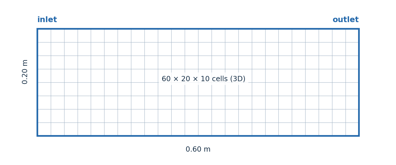
| cells | 60 × 20 × 10 | 12 000 |
| points | 61 × 21 × 11 | 14 091 |
| internal faces | 59·20·10 + 60·19·10 + 60·20·9 | 34 000 |
| inlet / outlet | 20 × 10 each | 200 + 200 |
| walls | 2·(60·10) + 2·(60·20) | 3 600 |
| total faces | 34 000 + 4 000 | 38 000 |
Consequently constant/polyMesh/boundary is expected to look like this (OpenFOAM may add entries such as inGroups):
3
(
    inlet
    {
        type            patch;
        nFaces          200;
        startFace       34000;
    }
    outlet
    {
        type            patch;
        nFaces          200;
        startFace       34200;
    }
    walls
    {
        type            wall;
        nFaces          3600;
        startFace       34400;
    }
)
Deep dive · Where discretisation error comes from and why it depends on cell shape
In OpenFOAM’s finite-volume method the unknowns are stored at cell centres and fluxes are computed on faces by interpolating the values of the two adjacent cells. Through Gauss’s theorem the cell gradient becomes a sum over faces: ∇φ ≈ (1/V)·Σ S_f·φ_f. A “second-order” scheme is really second order only if three geometric conditions hold: the centre-to-centre segment is parallel to the face normal (orthogonality), crosses the face at its centre (no skewness) and the two cells have similar sizes (volume ratio close to 1).
When one of these conditions fails, error terms proportional to the geometric deviation appear and they do not decrease with the square of the cell size: in practice the effective order drops towards 1. This is why checkMesh measures exactly non-orthogonality, skewness and volume ratios, and why in Guide 4 the observed order can come out lower than the nominal order of the schemes.
Deep dive · The exercise domain through an engineer’s eyes: blockage and distances
| Quantity | Value | Comment |
|---|---|---|
| blockage ratio | π·0.025² / (0.2·0.1) ≈ 9.8 % | in external aerodynamics one aims to stay below a few percent |
| upstream distance | 0.195 m ≈ 3.9 D | the uniform inlet is close to the obstacle |
| downstream distance | 0.355 m ≈ 7.1 D | short wake region for shedding studies |
| gap to the walls in z | 0.025 m = 0.5 D | strong confinement across the thickness |
| gap to the walls in y | 0.075 m = 1.5 D | — |
The case is meant for meshing practice, not for measuring the drag of an isolated sphere: with these ratios walls and outlet affect the field. In a real project the domain dimensions are decided before the mesh, based on the quantity to be measured, and checked with a sensitivity study on boundary placement, separate from the resolution study.
2. Prerequisites, tools and file formats
Assume OpenFOAM Foundation 14 on a Linux server, PowerShell and SSH for commands, FileZilla SFTP for file transfer, and Notepad++ for editing dictionaries on Windows. Use ParaView 5.13.2 via pvserver, as in Guides 1 and 3. No additional remote development editor is required.
This ZIP contains examples/01_channel_blockMesh/, examples/02_sphere_snappy/, the scripts/run_mesh_case.sh runner, and original figures. Upload the full exercise folder to a personal directory on the server without overwriting other cases. Shell scripts need Unix LF line endings, not Windows CRLF. In Notepad++, choose Edit → EOL Conversion → Unix (LF) and UTF-8 encoding.
ssh user@server.example
source /opt/OpenFOAM-14/etc/bashrc   # adjust installation path
foamVersion
cd ~/OpenFOAM
chmod +x mesh-guide6/scripts/run_mesh_case.sh
~/OpenFOAM/mesh-guide6 is an illustrative location: change it to the directory used after unzipping and transferring the materials. Coordinates in this guide are expressed in metres. An STL exported from a CAD system in millimetres does not automatically become a metre-based STL.
Deep dive · Checking the environment before every session
The meshing utilities belong to the same installation as the solver: if even one is missing, the environment has not been loaded or the installation is incomplete. The check takes a few seconds and avoids misleading errors halfway through.
source /opt/OpenFOAM-14/etc/bashrc
foamVersion
which blockMesh snappyHexMesh surfaceCheck checkMesh surfaceFeatures
echo "$WM_PROJECT_DIR"
# to load it at every login (adapt the path):
echo 'source /opt/OpenFOAM-14/etc/bashrc' >> ~/.bashrc
The STL file may be ASCII (text, starting with solid) or binary. SFTP always transfers bytes unchanged, so both arrive intact; line-ending conversion only concerns scripts and dictionaries edited with Notepad++. The empty mesh.foam file in both cases only lets ParaView recognise the directory as an OpenFOAM case.
Deep dive · ASCII or binary STL, and moving large meshes
The ASCII STL of the sphere takes 238,410 bytes for 896 triangles, about 266 bytes per triangle. The same content in binary format takes 80 + 4 + 50·896 = 44,884 bytes, five times less. For CAD surfaces with millions of triangles binary is mandatory; ASCII remains handy for teaching examples because it can be read in an editor. OpenFOAM reads both.
For large meshes polyMesh is not transferred file by file with FileZilla: compress it on the server and transfer a single archive, or do not transfer it at all and inspect the mesh via pvserver. In controlDict, writeFormat binary; and writeCompression on; reduce disk usage further.
tar czf sphere_mesh.tar.gz constant/polyMesh logs
du -sh constant/polyMesh sphere_mesh.tar.gz
3. Case structure and key files
| Path | Purpose | Typical change |
|---|---|---|
system/blockMeshDict | Vertices, blocks, grading and patches | Size and cell count |
system/snappyHexMeshDict | Surface refinement, snapping and layers | Meshing parameters |
system/controlDict | General run-time configuration | Usually minimal here |
constant/triSurface/*.stl | Triangulated geometric surfaces | CAD geometry |
constant/polyMesh/ | Mesh written by the utilities | Do not hand-edit |
logs/ | Evidence of preprocessing checks | Preserve for review |
The polyMesh directory stores points, faces, owner, neighbour and boundary: geometry, connectivity and boundary naming. These files should not be treated as editable CAD files. Their meaning is described in the official OpenFOAM 14 mesh-file documentation.
Deep dive · The complete controlDict of the meshing cases
Even though no equation is solved, the utilities read system/controlDict to know at which time to write, in which format and precision. The file is identical in the two examples:
/* OpenFOAM Foundation 14 - educational meshing example; GPL-3.0-or-later */
FoamFile
{
    version 2.0;
    format ascii;
    class dictionary;
    location "system";
    object controlDict;
}

application     foamRun;
startFrom       startTime;
startTime       0;
stopAt          endTime;
endTime         1;
deltaT          1;
writeControl    timeStep;
writeInterval   1;
purgeWrite      0;
writeFormat     ascii;
writePrecision  8;
writeCompression off;
timeFormat      general;
timePrecision   6;
runTimeModifiable true;
writeFormat asciikeeps thepolyMeshfiles readable in an editor; for large meshesbinaryreduces disk space and write time.writePrecision 8is the precision used for point coordinates: with large domains and small cells it should be increased, otherwise rounding can degrade the quality of very thin cells.application foamRunis not used by the meshing utilities: it is ready for when fields and physics are added to the case.
Deep dive · Sets and zones: what appears in polyMesh besides the mesh
constant/polyMesh/sets/: sets of cells, faces or points written for example bycheckMesh(the entities failing the checks) or bytopoSet. They are for diagnosis and for building zones; the solver does not use them directly.cellZones,faceZones,pointZones: named subsets that are part of the mesh and that the solver can use, for example for a porous medium, a localised source or a rotating zone.snappyHexMeshcan create them from closed surfaces withcellZoneandfaceZoneinrefinementSurfaces.- With
writeFormat asciithe first lines of each file give class and element count:head -n 25 constant/polyMesh/owneralso reports the number of points, cells and faces in its header.
4. Exercise A: a 3D channel with blockMesh
The first case generates a rectangular prism, 0.60 m long, 0.20 m high and 0.10 m deep, using 60 × 20 × 10 = 12,000 cells. The nominal cell width is 0.01 m in all three directions. Patches are named inlet, outlet and walls. This is a three-dimensional case, not a two-dimensional case using empty patches.
The supplied system/blockMeshDict contains:
scale 1;
vertices
(
    (0 0 0) (0.6 0 0) (0.6 0.2 0) (0 0.2 0)
    (0 0 0.1) (0.6 0 0.1) (0.6 0.2 0.1) (0 0.2 0.1)
);
blocks
(
    hex (0 1 2 3 4 5 6 7) (60 20 10)
    simpleGrading (1 1 1)
);
The outside faces must be assigned in boundary or explicitly handled. In the full example, the inlet face is (0 4 7 3), the outlet face is (1 2 6 5), and the other four faces belong to walls. Vertex ordering matters, because incorrect ordering may produce inverted blocks.
After uploading the exercise folder:
cd ~/OpenFOAM/mesh-guide6
./scripts/run_mesh_case.sh channel
The runner copies the template to a new directory under results/channel_..., generates the mesh and stores logs/log.blockMesh and logs/log.checkMesh.base. To learn the commands individually, work on a fresh copy of the template:
blockMesh -case /path/to/new-case-copy
checkMesh -case /path/to/new-case-copy \
    -allGeometry -allTopology
The expected blockMesh cell count is 12,000. If it differs, verify which input dictionary and case directory were actually used.
Further reading — nonuniform grading. simpleGrading (1 1 1) gives a uniform distribution. Different ratios allow concentration of cells near a surface or other region. Aggressive grading is not a substitute for proper local geometry resolution; abrupt size transitions may affect mesh quality and solver robustness.
Deep dive · The complete blockMeshDict and face orientation
/* OpenFOAM Foundation 14 - educational meshing example; GPL-3.0-or-later */
FoamFile
{
    version 2.0;
    format ascii;
    class dictionary;
    location "system";
    object blockMeshDict;
}

scale 1;

vertices
(
    (0 0 0)        // 0
    (0.6 0 0)      // 1
    (0.6 0.2 0)    // 2
    (0 0.2 0)      // 3
    (0 0 0.1)      // 4
    (0.6 0 0.1)    // 5
    (0.6 0.2 0.1)  // 6
    (0 0.2 0.1)    // 7
);

blocks
(
    hex (0 1 2 3 4 5 6 7) (60 20 10) simpleGrading (1 1 1)
);

edges ();

boundary
(
    inlet  { type patch; faces ((0 4 7 3)); }
    outlet { type patch; faces ((1 2 6 5)); }
    walls  { type wall;  faces ((0 1 5 4) (3 7 6 2) (0 3 2 1) (4 5 6 7)); }
);

mergePatchPairs ();
In the block hex (0 1 2 3 4 5 6 7) the first four vertices describe the bottom face and the last four the top face, in the same order; the sequence 0→1→2→3 must run anticlockwise when viewed from the side of vertices 4–7 (right-hand rule). The local axis x1 then runs from 0 to 1, x2 from 0 to 3, x3 from 0 to 4, and the three numbers (60 20 10) refer to these axes.
Boundary faces must be written so that the right-hand-rule normal points out of the block. Check on the inlet (0 4 7 3) face: with a = P4 − P0 = (0, 0, 0.1) and b = P7 − P4 = (0, 0.2, 0) the cross product is a × b = (−0.02, 0, 0), i.e. it points towards −x, out of the domain. If a face is written the wrong way round, blockMesh reports an error or produces an inconsistent orientation that checkMesh detects.
# numbers to compare with the table in section 1
grep -E "^\s*(points|faces|internal faces|cells):" results/channel_*/logs/log.checkMesh.base
grep -A3 "Patch" results/channel_*/logs/log.checkMesh.base
Deep dive · Grading: expansion ratio and first-cell size
In simpleGrading each number is the ratio between the last and the first cell along that axis. With n cells and total ratio E, cells grow geometrically with ratio r = E^(1/(n−1)) and the first cell is Δ₁ = L·(r − 1)/(rⁿ − 1).
Example on the channel: height L = 0.2 m, n = 20, E = 4. This gives r ≈ 1.0757, first cell Δ₁ ≈ 4.58 mm, last ≈ 18.3 mm. This, however, clusters cells at one wall only. To cluster at both walls use multi-section grading, where each triple gives (fraction of length, fraction of cells, expansion ratio):
hex (0 1 2 3 4 5 6 7) (60 20 10)
simpleGrading
(
    1
    ((0.5 0.5 4) (0.5 0.5 0.25))
    1
)
Each half (0.1 m, 10 cells) has r ≈ 1.1665: first wall cell ≈ 4.54 mm, centre cell ≈ 18.2 mm. A ratio between adjacent cells above roughly 1.2–1.3 tends to degrade the accuracy of second-order schemes: here it is 1.17, acceptable. For finer wall resolution, increase the number of cells, not just the ratio.
Deep dive · The same channel as a 2D case: empty patches and a single cell across the thickness
OpenFOAM always solves in 3D; a two-dimensional case is obtained with a single cell in the neglected direction and the two opposite faces of type empty. The exercise channel becomes:
blocks
(
    hex (0 1 2 3 4 5 6 7) (60 20 1) simpleGrading (1 1 1)
);

boundary
(
    inlet       { type patch; faces ((0 4 7 3)); }
    outlet      { type patch; faces ((1 2 6 5)); }
    walls       { type wall;  faces ((0 1 5 4) (3 7 6 2)); }
    frontAndBack
    {
        type empty;
        faces ((0 3 2 1) (4 5 6 7));
    }
);
Cells: 60 × 20 × 1 = 1,200. The empty patches receive no physical boundary conditions (fields use type empty;) and checkMesh recognises the case as 2D. For an axisymmetric case use a wedge with wedge patches of a few degrees instead. symmetryPlane and symmetry patches are for physical symmetry planes, not for reducing dimensionality.
Deep dive · Multiple blocks, curved edges and topology checks
More complex geometries are built with several blocks sharing vertices: coincident faces are merged automatically, provided the cell counts on the shared edges match. Curved edges are described in the edges list, for example with an arc through three points:
edges
(
    // arc from vertex 1 to vertex 2 through the intermediate point
    arc 1 2 (0.65 0.1 0)
    arc 5 6 (0.65 0.1 0.1)   // the same arc on the opposite face
);
Before generating the mesh it is worth checking blocks, numbering and faces with the option that writes only the block topology, to be opened in ParaView; a wrong vertex shows up immediately as a twisted block:
blockMesh -blockTopology
ls *.obj        # block-topology files, can be opened in ParaView
blockMesh -help
5. Moving from CAD geometry to an STL surface
Exercise B includes a closed sphere STL with radius 0.025 m and centre (0.22, 0.10, 0.05) m, embedded in the same channel. The STL file is included: Python is not required on the Linux server to run the exercise.
When working with FreeCAD or another CAD tool:
- Define the intended physical size and verify units after exporting.
- Ensure the solid-bounding surface is closed and consistently oriented; check for holes, duplicate faces and self-intersections.
- Export an STL with enough surface triangles to resolve the features of interest.
- Upload it to
constant/triSurface/using FileZilla. - Run
surfaceCheckand inspect the bounding box and surface connectivity.
surfaceCheck constant/triSurface/sphere.stlRun this command from the case directory (or provide an absolute STL path). STL does not carry reliable unit metadata. surfaceCheck is a useful way to detect coordinates incompatible with the background domain. For example, a 25 mm part exported as 25 units and then interpreted as metres becomes 1,000 times too large.
Refresher — geometric versus mesh accuracy. Refining the volume cells does not remove an error already introduced by an overly coarse STL approximation. Keep the CAD surface tessellation and CFD cell-size requirements separate.
Deep dive · Measuring the STL before using it: volume, area, edge length
This script, standard Python library only, reads an ASCII STL and computes the bounding box, area, enclosed volume (divergence theorem) and triangle edge lengths. It runs on the server or on Windows:
#!/usr/bin/env python3
"""Bounding box, area, enclosed volume and edge lengths of an ASCII STL (standard library only)."""
import math, sys

tri, cur = [], []
with open(sys.argv[1], encoding="utf-8", errors="replace") as f:
    for line in f:
        w = line.split()
        if w and w[0] == "vertex":
            cur.append(tuple(map(float, w[1:4])))
        elif w and w[0] == "endloop":
            tri.append(cur); cur = []

lo, hi = [math.inf] * 3, [-math.inf] * 3
vol = area = 0.0
edges = []
for a, b, c in tri:
    for p in (a, b, c):
        lo = [min(lo[i], p[i]) for i in range(3)]
        hi = [max(hi[i], p[i]) for i in range(3)]
    # signed volume of the tetrahedron (origin, a, b, c): divergence theorem
    vol += (a[0]*(b[1]*c[2]-b[2]*c[1]) - a[1]*(b[0]*c[2]-b[2]*c[0]) + a[2]*(b[0]*c[1]-b[1]*c[0])) / 6
    u = [b[i]-a[i] for i in range(3)]; v = [c[i]-a[i] for i in range(3)]
    n = (u[1]*v[2]-u[2]*v[1], u[2]*v[0]-u[0]*v[2], u[0]*v[1]-u[1]*v[0])
    area += 0.5 * math.sqrt(sum(x*x for x in n))
    edges += [math.dist(a, b), math.dist(b, c), math.dist(c, a)]

print(f"triangles     {len(tri)}")
print(f"bounding box  {lo} -> {hi}")
print(f"area          {area:.6e}")
print(f"volume        {vol:.6e}   (negative = normals pointing inwards)")
print(f"edge length   min {min(edges):.3e}  mean {sum(edges)/len(edges):.3e}  max {max(edges):.3e}")
python3 stl_info.py constant/triSurface/sphere.stlOn the package sphere (896 triangles) the values are:
| Quantity | STL | Exact sphere, r = 0.025 m | Difference |
|---|---|---|---|
| bounding box x | 0.19514 … 0.24486 | 0.195 … 0.245 | — |
| bounding box z | 0.025 … 0.075 | 0.025 … 0.075 | — |
| area [m²] | 7.786·10⁻³ | 7.854·10⁻³ | −0.87 % |
| volume [m³] | 6.432·10⁻⁵ | 6.545·10⁻⁵ | −1.73 % |
| mean edge [mm] | 4.95 (min 1.02, max 7.15) | — | — |
The STL is an inscribed polyhedron: volume and area are slightly smaller than those of the true sphere, and in x and y the bounding box does not reach ±0.025 because no vertex lies exactly on the equator in those directions. This is the geometric error mentioned in the refresher: no mesh refinement removes it. The expected fluid volume is therefore 0.012 − 6.432·10⁻⁵ ≈ 0.011936 m³, to be compared with the “Total volume” reported by checkMesh. A negative volume would indicate triangles with inward-pointing normals.
Deep dive · Wrong units: rescaling the STL without going back to the CAD
If surfaceCheck shows a bounding box a thousand times too large (CAD in millimetres), the surface can be rescaled with surfaceTransformPoints, writing a new file and leaving the original untouched. The transformation syntax has changed between versions: check the one of your installation with -help.
surfaceTransformPoints -help
# form used in recent Foundation versions:
surfaceTransformPoints "scale=(0.001 0.001 0.001)" \
    constant/triSurface/part_mm.stl constant/triSurface/part_m.stl
surfaceCheck constant/triSurface/part_m.stl
In the surfaceCheck output look for the bounding box, the statement that the surface is closed (every edge shared by two triangles) and the absence of illegal triangles or intersections. A non-closed STL can still be used by snappyHexMesh, but the separation between fluid and solid becomes unreliable: the fluid can “leak” through the hole and the region to be removed is no longer recognised.
Deep dive · Export tolerance: how far the STL departs from the true surface
For a triangle edge s on a surface of curvature radius R, the maximum distance between chord and arc (sagitta) is about δ ≈ s² / (8R). CAD tools call this parameter “deviation” or “chordal tolerance” in the STL export.
| Triangle edge | δ = s²/(8·0.025 m) | Relative to the level-2 cell (2.5 mm) |
|---|---|---|
| 4.95 mm (mean) | ≈ 0.12 mm | ≈ 5 % |
| 7.15 mm (max) | ≈ 0.26 mm | ≈ 10 % |
Rule of thumb: the STL deviation must be small compared with the finest cell planned on the surface and with the wall thicknesses of interest. If wall layers of tenths of a millimetre are planned, a 0.26 mm sagitta is too large: export with a tighter tolerance.
Deep dive · An STL with several regions to obtain separate patches
An ASCII STL can contain several solid name … endsolid name blocks. snappyHexMesh treats them as regions of the same surface and can give each a different level and patch type: this is the proper way to get separate inlet, outlet and walls from a single CAD file. Name each face group at export; in snappyHexMeshDict:
refinementSurfaces
{
    part.stl
    {
        level (2 2);
        regions
        {
            inlet  { level (2 2); patchInfo { type patch; } }
            outlet { level (2 2); patchInfo { type patch; } }
            walls  { level (2 3); patchInfo { type wall;  } }
        }
    }
}
The resulting patch names combine geometry and region names; read them in constant/polyMesh/boundary and use them verbatim in the fields in 0/. surfaceCheck lists the regions present in the file.
6. Exercise B: snappyHexMesh around a sphere
snappyHexMesh starts from a hexahedral background grid and performs castellation, snapping, and optionally boundary-layer addition. The supplied exercise deliberately disables layers so that the solid surface and fluid-region selection can be tested first.
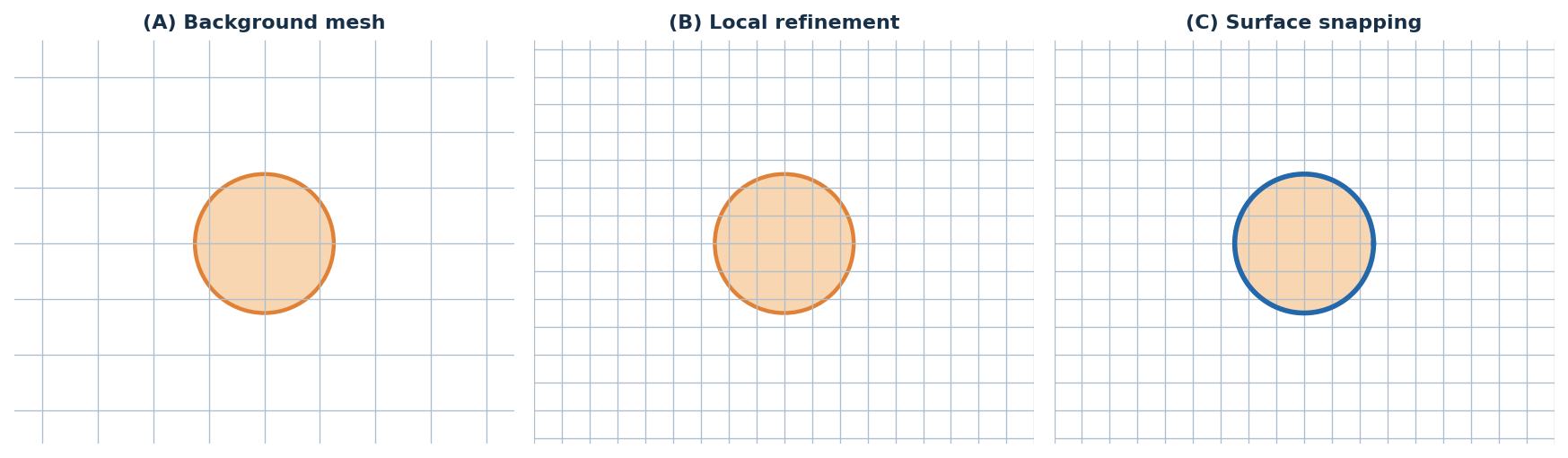
The full system/snappyHexMeshDict includes these entries:
castellatedMesh true;
snap            true;
addLayers       false;

geometry
{
    sphere.stl { type triSurfaceMesh; }
}

castellatedMeshControls
{
    // See the full dictionary for additional controls
    refinementSurfaces
    {
        sphere.stl { level (2 2); patchInfo { type wall; } }
    }
    locationInMesh (0.517 0.113 0.057);
}
The locationInMesh point must lie inside the fluid volume to retain: not inside the sphere, not on its triangulated surface, and not exactly on a background mesh face. The wrong point can cause the intended region to be removed. The supplied features (); and implicit feature snapping work as a teaching example for a smooth sphere. For CAD with sharp edges, feature-edge extraction through surfaceFeatures may be useful, as documented in the Foundation guide.
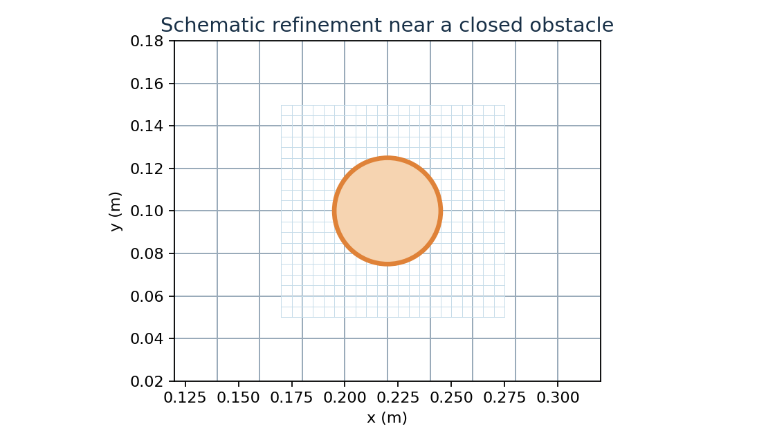
Generate the mesh using:
cd ~/OpenFOAM/mesh-guide6
./scripts/run_mesh_case.sh sphere
The runner creates results/sphere_..., performs blockMesh, an initial checkMesh, surfaceCheck, snappyHexMesh -overwrite on the newly copied case only, and a final checkMesh. Here -overwrite replaces the background polyMesh in the fresh working copy; it does not affect the source templates. Never run this command on an existing published result without an appropriate working copy.
If a command fails, read its corresponding file under logs/. Investigate STL defects first if surfaceCheck fails. If snappyHexMesh fails, review fluid-region selection, near-surface clearance, refinement settings and cell quality.
Deep dive · The complete snappyHexMeshDict, entry by entry
/* OpenFOAM Foundation 14 - educational meshing example; GPL-3.0-or-later */
FoamFile
{
    version 2.0;
    format ascii;
    class dictionary;
    location "system";
    object snappyHexMeshDict;
}

castellatedMesh true;
snap            true;
addLayers       false; // optional extension: see the guide

geometry
{
    sphere.stl
    {
        type triSurfaceMesh;
    }
}

castellatedMeshControls
{
    maxLocalCells       150000;
    maxGlobalCells      350000;
    minRefinementCells  0;
    maxLoadUnbalance    0.10;
    nCellsBetweenLevels 3;

    features ();

    refinementSurfaces
    {
        sphere.stl
        {
            level (2 2);
            patchInfo { type wall; }
        }
    }
    resolveFeatureAngle 30;
    refinementRegions {};
    locationInMesh (0.517 0.113 0.057); // fluid region; not on a face
    allowFreeStandingZoneFaces true;
}

snapControls
{
    nSmoothPatch       3;
    tolerance          2.0;
    nSolveIter         30;
    nRelaxIter         5;
    nFeatureSnapIter   10;
    implicitFeatureSnap true;
    explicitFeatureSnap false;
    multiRegionFeatureSnap false;
}

// Layers are off in the main exercise. Add them only after a clean base mesh.
addLayersControls
{
    relativeSizes true;
    layers {};
    expansionRatio 1.2;
    finalLayerThickness 0.3;
    minThickness 0.1;
    nGrow 0;
    featureAngle 60;
    nRelaxIter 5;
    nSmoothSurfaceNormals 1;
    nSmoothNormals 3;
    nSmoothThickness 10;
    maxFaceThicknessRatio 0.5;
    maxThicknessToMedialRatio 0.3;
    minMedianAxisAngle 90;
    nBufferCellsNoExtrude 0;
    nLayerIter 50;
}

meshQualityControls
{
    maxNonOrtho          65;
    maxBoundarySkewness  20;
    maxInternalSkewness  4;
    maxConcave           80;
    minVol               1e-13;
    minTetQuality        -1e30;
    minArea              -1;
    minTwist             0.02;
    minDeterminant       0.001;
    minFaceWeight        0.02;
    minVolRatio          0.01;
    minTriangleTwist     -1;
    nSmoothScale         4;
    errorReduction       0.75;
}

mergeTolerance 1e-6;| Entry | What it does |
|---|---|
maxLocalCells / maxGlobalCells | cell limit per processor and in total during refinement; beyond the latter, refinement stops before the requested level |
minRefinementCells | if fewer cells than this are marked for refinement, the refinement loop ends |
nCellsBetweenLevels | cell layers between two refinement levels: higher = smoother transition |
resolveFeatureAngle | where the angle between surface normals exceeds this value, cells are refined up to the maximum level |
level (2 2) | minimum and maximum level on the surface; the maximum applies where curvature exceeds resolveFeatureAngle |
tolerance 2.0 | maximum distance, in multiples of the local cell size, within which a point is attracted onto the surface |
nSmoothPatch, nSolveIter, nRelaxIter | iterations of surface smoothing, displacement relaxation and bad-cell correction |
implicitFeatureSnap | detects edges from the surface itself, without a feature file |
meshQualityControls | limits that snapping and layers must not violate; a change that violates them is undone locally |
mergeTolerance | tolerance, relative to the domain extent, used to merge coincident points |
Deep dive · The refinement arithmetic around the sphere and the choice of the inside point
The background mesh has 10 mm cells. Each level halves the edge length: level 1 = 5 mm, level 2 = 2.5 mm. The sphere is 50 mm in diameter, so it spans 5 background cells but about 20 cells at level 2; the circumference (≈ 157 mm) is described by about 63 cells. The mean STL triangle edge is about 4.9 mm: with 2.5 mm cells the mesh “sees” the facets of the polyhedron, so refining further without a finer STL does not bring the surface closer to a true sphere.
The point (0.517 0.113 0.057) was chosen deliberately: it is about 0.297 m from the sphere centre, so it is in the fluid; none of its coordinates is a multiple of 10 mm, 2.5 mm or 1.25 mm (0.517/0.0025 = 206.8), so it does not lie on a face even after refinement. Choosing “irregular” coordinates is good practice for exactly this reason.
In more recent OpenFOAM Foundation versions the same entry also appears in the tutorials as insidePoint. To find out which form your installation uses, search the tutorials:
grep -rl --include=snappyHexMeshDict -E "insidePoint|locationInMesh" "$FOAM_TUTORIALS" | head
grep -rh --include=snappyHexMeshDict -E "^\s*(insidePoint|locationInMesh)" "$FOAM_TUTORIALS" | sort | uniq -c
Deep dive · Seeing the three stages separately: without -overwrite
Without -overwrite, snappyHexMesh writes each stage into a separate time directory: the castellated mesh in the first, the snapped mesh in the second and, if enabled, the layers in the third; the background mesh stays in constant/polyMesh. Opening the case in ParaView and stepping through the times shows the effect of each stage. Do this in a dedicated copy, never in the case the simulation will start from.
cp -a examples/02_sphere_snappy "$HOME/mesh-runs/sphere_stages"
cd "$HOME/mesh-runs/sphere_stages"
blockMesh > log.blockMesh 2>&1
snappyHexMesh > log.snappyHexMesh 2>&1
ls -d [0-9]*/        # one directory per stage
Deep dive · Sharp edges: extracting feature edges with surfaceFeatures
The sphere has no edges, which is why the dictionary uses features (); and implicit snapping. A CAD part with sharp edges (flanges, steps, leading edges) instead requires the mesh to follow the edge lines, otherwise edges come out rounded. In OpenFOAM Foundation extraction is done with surfaceFeatures, which reads system/surfaceFeaturesDict and writes an .eMesh file into constant/. A minimal dictionary:
FoamFile
{
    format      ascii;
    class       dictionary;
    object      surfaceFeaturesDict;
}

surfaces ("part.stl");

// keeps edges where faces meet at less than 150°
includedAngle   150;
Then in snappyHexMeshDict list the files in features ( { file "part.eMesh"; level 2; } ); and enable explicitFeatureSnap true; (usually with implicitFeatureSnap false;). The motorBike tutorial in your installation shows the complete sequence.
Deep dive · What really happens in castellation, snapping and layers
- Castellation: background cells cut by the surface, or close to features and regions, are split into 8 up to the requested level, honouring
nCellsBetweenLevels. Cells are then classified against the surface and only the region connected to the inside point is kept; the separating faces become the patch. The result is a stair-stepped mesh, still all hexahedra. - Snapping: the points of the stair-stepped patch are projected onto the surface (within
tolerancetimes the local size), and the displacement is propagated inwards by solving a relaxation problem. Where a cell violatesmeshQualityControls, the displacement is scaled back locally (errorReduction,nSmoothScale). Cells near the surface become polyhedra. - Layers: the mesh is “shrunk” away from the wall and the freed space is filled with prisms extruded along the normals. Where extrusion would violate the quality controls, layers are reduced or removed locally: that is why actual coverage must always be checked.
Two practical rules follow from this: the background mesh should have cells as cubic as possible (aspect ratio close to 1), otherwise refinement produces stretched cells and snapping degrades; and the background cell must be small enough relative to the details that, after refinement, every fluid gap contains several cells.
Deep dive · snappyHexMesh quality controls, entry by entry
| Entry (package value) | What it limits |
|---|---|
maxNonOrtho 65 | maximum angle between face normal and centre-to-centre line, in degrees |
maxBoundarySkewness 20 / maxInternalSkewness 4 | maximum skewness on boundary and internal faces |
maxConcave 80 | maximum concavity angle of a face |
minVol 1e-13 | minimum cell volume: excludes degenerate or inverted cells |
minTetQuality -1e30 | minimum quality of the tetrahedral decomposition; the very negative value disables the check |
minArea -1 | minimum face area; negative = disabled |
minTwist 0.02 | minimum twist: alignment between the face normal and those of its triangles |
minDeterminant 0.001 | cell determinant (1 for a perfect hexahedron): small values indicate flattened cells |
minFaceWeight 0.02 | face interpolation weight (0–0.5): small values mean very different adjacent cells |
minVolRatio 0.01 | minimum volume ratio between adjacent cells |
minTriangleTwist -1 | triangle twist; negative = disabled |
nSmoothScale 4, errorReduction 0.75 | iterations and factor by which displacement is scaled back where limits are violated |
Loosening these limits makes snappy “pass” but moves the problem onto the solver. The right direction is usually another: a more regular background mesh, a different level or snap tolerance, a cleaner STL.
Deep dive · Reading log.snappyHexMesh without getting lost
The log is long; an engineering check needs only a few items: cell count after each refinement loop, cells removed by region selection, morphing iterations and cells violating the controls, the layer table if any, and total time.
grep -n -E "Refinement phase|Surface refinement iteration|Removing|cells:|Morph iteration|Snapped mesh|Layer|Finished meshing|ExecutionTime" logs/log.snappyHexMesh | tail -n 60
grep -n -i -E "warning|error|illegal" logs/log.snappyHexMesh
A cell count that stops growing before the requested level, together with a value close to maxGlobalCells, indicates truncated refinement; many cells violating the controls after the last morph iteration indicate incomplete snapping.
Deep dive · Generating the mesh in parallel
For large meshes snappyHexMesh runs in parallel like a solver: decompose the background mesh, run with -parallel and the simulation can start directly on the decomposed case, without reconstructing. The number of subdomains in system/decomposeParDict must match the number of processes (see Guide 5).
blockMesh
decomposePar
mpirun -np 4 snappyHexMesh -parallel -overwrite > logs/log.snappyHexMesh 2>&1
mpirun -np 4 checkMesh -parallel -allGeometry -allTopology > logs/log.checkMesh.final 2>&1
# to gather the mesh into a single case, check the options of your version:
reconstructPar -help
Load balancing during refinement is controlled by maxLoadUnbalance (0.10 in the package): beyond this imbalance between processors the mesh is redistributed.
7. Important snappyHexMesh controls
| Entry | Practical meaning | Common issue |
|---|---|---|
refinementSurfaces.level (2 2) | Two surface-refinement levels | Too many or too few cells |
nCellsBetweenLevels | Transition between refinement levels | Abrupt size changes |
maxGlobalCells | Global cell-count limit | Refinement stops early |
locationInMesh | Point identifying fluid to keep | Wrong region removed |
snapControls | Morph grid to target surface | Poor fit or distorted cells |
addLayers | Enable near-wall layers | Requested layers not obtained |
meshQualityControls | Meshing quality thresholds | Poor cells may slip through |
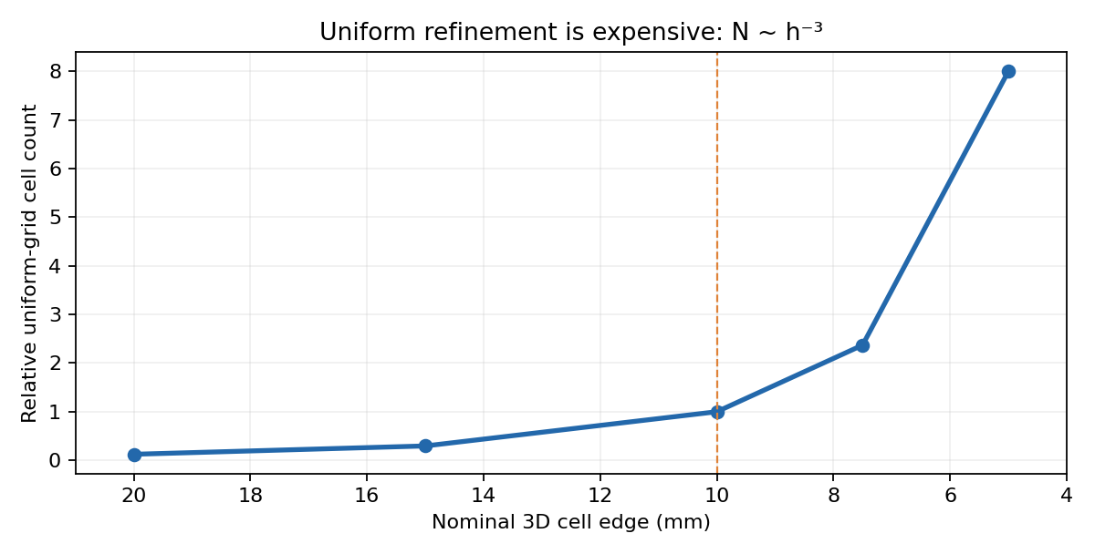
One refinement level approximately halves the local cell edge length. If an entire 3D region is uniformly refined, this can increase cell count by a factor of approximately eight per level. Refine where geometry and physics actually require it.
Deep dive · Refining a region: the wake behind the sphere
Besides the surface, a volume can be refined. Auxiliary geometries are declared in geometry and used in refinementRegions in three modes: inside, outside or distance (levels as a function of the distance from a surface). Example for a wake about 9 diameters long:
geometry
{
    sphere.stl { type triSurfaceMesh; }
    wakeBox
    {
        type box;              // in older versions: searchableBox
        min  (0.20 0.07 0.02);
        max  (0.60 0.13 0.08);
    }
}

castellatedMeshControls
{
    // ...
    refinementRegions
    {
        wakeBox    { mode inside;   levels ((1E15 1)); }
        sphere.stl { mode distance; levels ((0.01 2) (0.03 1)); }
    }
}
In distance mode the (distance, level) pairs go in order of increasing distance and decreasing level: here level 2 within 10 mm of the sphere and level 1 within 30 mm. The geometry type name must be checked in your version, for example with grep -rh --include=snappyHexMeshDict "type *[a-zA-Z]*Box\|type *box" "$FOAM_TUTORIALS" | sort | uniq -c.
Deep dive · How many cells a level costs
In 3D each level splits a cell into 8: a region fully refined to level L costs 8^L times the original cells. The channel has 12 000 background cells: uniformly refined it would become 96 000 cells at level 1, 768 000 at level 2, more than 6 million at level 3. Local refinement exists precisely to avoid this growth: the cost depends on the refined area, not on the domain volume.
For the surface alone the order of magnitude is area / Δ² cells per layer: the sphere (7.8·10⁻³ m²) with 2.5 mm cells needs about 1 250 cells per layer, plus the transition layers imposed by nCellsBetweenLevels. The actual number is at the end of log.snappyHexMesh and must be compared with maxGlobalCells: if it is close to the limit, refinement may have been truncated.
Deep dive · Memory and time: measure them instead of guessing
The memory needed by snappyHexMesh grows with cell count and surface complexity; literature and forums quote orders of magnitude of roughly one gigabyte per million cells, but the figure that matters is the one measured on your own server with a smaller pilot mesh, extrapolated linearly before launching the final one.
/usr/bin/time -v snappyHexMesh -overwrite > logs/log.snappyHexMesh 2> logs/time.snappyHexMesh
grep -E "Maximum resident set size|Elapsed" logs/time.snappyHexMesh
grep -E "^\s*cells:" logs/log.checkMesh.final
The ratio between peak memory and cell count of the pilot mesh, multiplied by the expected cell count, gives a reliable estimate; if it exceeds the node’s free RAM, the mesh must be generated in parallel on more processes or with a lower level.
8. Boundary layers and y+ considerations
Prismatic boundary layers are important when the turbulence model and required observables need near-wall resolution. Introduce them only after the base mesh is acceptable. addLayers false; is intentional in the supplied example.
A preliminary estimate of the wall-coordinate value at the first cell centre is:
Equation: y⁺ = (uτ · y) / ν, where uτ = √(τw / ρ).
Here y is the actual distance from the wall to the cell centre, not necessarily the specified thickness of the first generated layer. Suitable targets depend on the physical model, wall treatment and simulation objective; there is no universal target value. Check the number and coverage of layers actually produced, not just the number requested in the dictionary.
Refresher — why is y+ not solely a mesh property? It depends on local wall shear stress, which comes from the flow solution. Before solving, use an engineering estimate; afterwards, examine the actual distribution.
Deep dive · Estimating the first-layer thickness: a worked example
Before the run, τw is estimated with a turbulent flat-plate correlation, for example Cf ≈ 0.0592·Re_x^(−1/5), with τw = ½·ρ·U²·Cf. It is an order-of-magnitude estimate, to be checked on the computed field.
| Step | Water, U = 1 m/s, x = 0.2 m, ν = 10⁻⁶ m²/s |
|---|---|
| Re_x = U·x/ν | 2·10⁵ |
| Cf | ≈ 5.15·10⁻³ |
| τw = ½·ρ·U²·Cf | ≈ 2.58 Pa |
| uτ = √(τw/ρ) | ≈ 0.0508 m/s |
| y for y⁺ = 1 | ≈ 0.020 mm |
| y for y⁺ = 30 | ≈ 0.59 mm |
Since y is the distance of the first cell centre, the first-layer thickness is about 2·y. The difference between the last two rows (a factor of 30) explains why the wall treatment, resolved or with wall functions, must be chosen before building layers. At much lower velocities the flow may be laminar and the turbulent estimate does not apply.
Deep dive · Enabling layers on the sphere and checking what was obtained
Starting from a fresh copy of the case, layers are enabled with addLayers true; and by listing the patches in addLayersControls/layers. The name of the patch created on the sphere is in constant/polyMesh/boundary after the first snappyHexMesh; a regular expression avoids having to guess it:
addLayers       true;

addLayersControls
{
    relativeSizes       true;
    layers
    {
        "sphere.*" { nSurfaceLayers 3; }
    }
    expansionRatio      1.2;
    finalLayerThickness 0.3;
    minThickness        0.1;
    // the other entries stay as in the supplied file
}
With relativeSizes true thicknesses are fractions of the adjacent cell: here the last layer is 30 % of the 2.5 mm cell. At the end of the layering stage the log reports, for each patch, how many faces received layers and the average thickness obtained: if coverage is low, the requested layers do not really exist in those areas, and y⁺ must be assessed on the actual mesh.
Deep dive · Total layer thickness and the jump to the first outer cell
With first layer t₁, expansion ratio r and n layers, the total thickness is T = t₁·(rⁿ − 1)/(r − 1) and the last layer is t₁·r^(n−1). Example for y⁺ ≈ 1 in water at 1 m/s (first cell centre at about 0.02 mm, hence t₁ ≈ 0.04 mm), with r = 1.2 and n = 10:
| Quantity | Value |
|---|---|
| total thickness T | ≈ 1.04 mm |
| last layer | ≈ 0.21 mm |
| outer cell at level 2 | 2.5 mm |
| last layer / outer cell ratio | ≈ 0.08 |
A more than tenfold jump between the last layer and the outer cell is a resolution discontinuity that degrades gradients and fluxes precisely where it matters most. Possible fixes: more layers, a somewhat higher expansion ratio, a finer surface level (smaller outer cell), or a wall-function treatment with a thicker first layer.
Typical ranges, to be checked for the model in use: low-Reynolds models resolving the viscous sublayer with y⁺ of order 1; standard wall functions with the first cell centre in the log region, typically between about 30 and a few hundred. The buffer region (about 5–30) is to be avoided with classical wall functions.
Deep dive · The addLayersControls entries
| Entry | Meaning |
|---|---|
relativeSizes | thicknesses as a fraction of the adjacent cell (true) or in metres (false) |
expansionRatio | ratio between consecutive layer thicknesses |
finalLayerThickness | thickness of the last layer (furthest from the wall) |
minThickness | thickness below which the layer is not created |
nGrow | edge faces left without layers to ease the transition near adjacent patches |
featureAngle | angle beyond which extrusion stops at edges |
nSmoothSurfaceNormals, nSmoothNormals, nSmoothThickness | smoothing of extrusion normals and thickness |
maxFaceThicknessRatio | reduces layers on highly warped faces |
maxThicknessToMedialRatio, minMedianAxisAngle | limit layers in narrow gaps, where two walls approach each other |
nBufferCellsNoExtrude | buffer cells between areas with and without layers |
nLayerIter, nRelaxIter | maximum iterations for layer addition and relaxation |
9. Reading checkMesh results
checkMesh performs geometric and topological consistency checks. It does not establish whether the simulated physics is accurate. The exercise runs the extended checks:
checkMesh -case /path/to/case -allGeometry -allTopologyThree different classes of evidence must be distinguished:
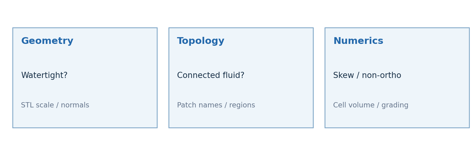
- Topology: disconnected fluid components, problematic faces or cells, invalid regions.
- Geometry: skewness, non-orthogonality, very small or negative cell volumes, degeneracies.
- Scientific suitability: resolution of physical gradients, wakes and boundary layers; this requires additional analyses.
Do not use one rigid threshold as a universal rule for every solver. A highly non-orthogonal mesh can require special numerical treatment, while a small number of damaged cells in a sensitive region can matter more than many mediocre cells elsewhere. Record cell count, extrema of relevant metrics, violation counts and problem locations.
Deep dive · What non-orthogonality, skewness and aspect ratio measure
- Non-orthogonality: angle between a face normal and the segment joining the two cell centres. At 0° the normal gradient is computed exactly from the two cell values; as the angle grows a correction is needed (
nNonOrthogonalCorrectorsinfvSolution,corrected/limitedschemes infvSchemes).checkMeshflags faces above 70° as severe. - Skewness: normalised distance between the point where the centre-to-centre segment crosses the face and the face centre. It introduces an error when interpolating values to the face. The
checkMeshreporting thresholds are 4 for internal faces and 20 for boundary faces, the same values used bymaxInternalSkewnessandmaxBoundarySkewnessin the snappy dictionary. - Aspect ratio: ratio between the largest and smallest cell dimension. High values are normal and intended in wall layers; they become a problem when the stretching is not aligned with the gradient direction.
- Regions:
checkMeshcounts connected regions. More than one region means part of the domain does not communicate with the rest: in the sphere case, an interior that was not removed.
For the uniform block channel the expected values are: maximum non-orthogonality 0, skewness practically zero, aspect ratio 1 (10 mm cubic cells), total volume 0.012 m³, a single region, “Mesh OK.”. Any deviation means you are not looking at the case you think.
Deep dive · Extracting the numbers from the logs and locating bad cells
This script summarises all the checkMesh logs produced by run_mesh_case.sh: run it from the package folder and copy the result into the table in section 12.
#!/usr/bin/env bash
# Summarise the key numbers of every checkMesh log under a results directory.
for f in "${1:-results}"/*/logs/log.checkMesh.*; do
  echo "== $f"
  grep -E "^\s*(points|faces|internal faces|cells):" "$f"
  grep -E "Overall domain bounding box|Total volume|Max aspect ratio|Mesh non-orthogonality|Max skewness" "$f"
  grep -E "\*\*\*|Mesh OK|Failed [0-9]+ mesh checks" "$f"
done
Lines starting with *** are failed checks; checkMesh also writes the sets of problematic faces and cells into constant/polyMesh/sets/, which can be shown in ParaView by enabling sets in the reader to see where they are. To write quality fields to colour in ParaView, check the available options with checkMesh -help.
Deep dive · From checkMesh diagnostics to choices in fvSchemes and fvSolution
The maximum non-orthogonality reported by checkMesh directly guides the numerical settings. A widespread practice, to be adapted to the case:
| Max non-orthogonality | laplacianSchemes / snGradSchemes | nNonOrthogonalCorrectors |
|---|---|---|
| < 60° | Gauss linear corrected / corrected | 0 |
| 60°–70° | Gauss linear corrected / corrected | 1 |
| 70°–80° | Gauss linear limited corrected 0.5 / limited corrected 0.5 | 1–2 |
| > 80° | revise the mesh | — |
With limited the non-orthogonal correction is limited for stability, at the expense of accuracy: a deliberate compromise to be documented. High skewness is partly compensated by limited gradient schemes (cellLimited Gauss linear 1) but the real remedy is geometric. Parts 5 and 6 of the path cover fvSchemes and fvSolution in detail.
Deep dive · Making the check automatic: fail when the mesh fails
In an automated chain (Guide 5) a mesh that fails the checks should stop the procedure rather than produce a run to be thrown away. The check is done on the log text:
log=logs/log.checkMesh.final
if grep -q "Mesh OK" "$log"; then
    echo "mesh accepted"
else
    grep -E "\*\*\*|Failed" "$log"
    echo "mesh rejected: see $log" >&2
    exit 3
fi
Some versions also offer a check against thresholds defined in a dedicated dictionary (checkMesh -meshQuality, which reads system/meshQualityDict): check availability with checkMesh -help and, if present, use the same limits as meshQualityControls.
10. Inspecting the mesh from Windows
Connect ParaView on Windows to pvserver as shown in Guide 1. Using the server-side file browser, find the generated case and open mesh.foam. Enable the desired mesh regions and patches in the reader, click Apply, then choose Surface With Edges. Use Slice to examine interior refinement and Extract Surface to inspect the sphere. The CFD data remain on the server: when working over pvserver, there is no need to download the full polyMesh directory just to display it.
Confirm that inlet, outlet, walls and the sphere patch exist, that sphere-interior cells have been excluded, and that local refinement occurs where expected. Images in this guide are original explanatory diagrams, not actual screenshots from ParaView.
Deep dive · Quantitative checks in ParaView, beyond the eye
- Fluid volume:
Integrate Variableson the internal region returns the volume; for the sphere it should be close to 0.011936 m³ (value computed from the STL in section 5). - Whole cells: a
Clipwith the Crinkle clip option shows whole cells instead of cutting them, revealing refinement levels and transitions. - Patches: in the reader panel, under Mesh Regions, select only the sphere patch to compare its faces with the original STL, loaded as a second file.
- Polyhedra: snappy creates polyhedral cells near the surface; the reader option that decomposes polyhedra changes only the display, not the mesh used by the solver.
Deep dive · ParaView’s Mesh Quality filter and quality maps
ParaView provides the Mesh Quality filter, which computes per-cell metrics such as aspect ratio, skew or scaled Jacobian for hexahedra and tetrahedra; on the general polyhedra produced by snappy many metrics are undefined. It is therefore more reliable to colour the mesh with the fields or sets written by checkMesh, which use the same definitions as the solver. To locate the worst cells: Threshold on the quality field, then Extract Cells By Region or a Clip with Crinkle clip around the area.
11. Three diagnostic scenarios
A. The sphere is enormous, or the mesh never intersects it. Compare the surfaceCheck bounding box against the blockMesh domain. This commonly indicates incorrect CAD units or coordinates.
B. Only the solid interior is retained, or the fluid region disappears. Inspect locationInMesh and STL integrity. A point on a background-grid face or boundary is not a robust identifier of the fluid region.
C. A mesh is produced but contains poor cells near the obstacle. Refinement levels, size transitions, snap tolerances, obstacle size relative to background cells and STL tessellation all interact. Change one parameter at a time, generate a separate case and compare logs.
Deep dive · Quick commands for the three scenarios
# A. bounding box comparison
grep -i "bounding box" logs/log.surfaceCheck logs/log.checkMesh.base

# B. how many regions remain and which volume
grep -E "regions|Total volume" logs/log.checkMesh.final

# C. failed checks and flagged cells
grep -E "\*\*\*|Failed|severely" logs/log.checkMesh.final
ls constant/polyMesh/sets/ 2>/dev/null
For scenario B the volume is the quickest check: if the retained region were the inside of the sphere, the volume would be about 6.4·10⁻⁵ m³ instead of about 0.0119 m³.
Deep dive · Two more typical failures: a leaking region and an inside point outside the domain
- D. The fluid “passes through” the solid. If the STL has a hole larger than the cells at the level reached, inside and outside become connected: the cavity is not removed and the domain volume equals that of the full channel (0.012 m³). Remedy: close the surface (
surfaceCheckreports open edges), do not raise the level. - E. The inside point is not in the mesh. If
locationInMeshfalls outside the background-mesh bounding box (for example because the geometry was rescaled or moved),snappyHexMeshstops with a fatal error mentioning the point. Remedy: recompute the point in the new coordinates and check it against theblockMeshbounding box.
12. A minimum pre-solver acceptance plan
| Check | Preserve this evidence | Acceptance question |
|---|---|---|
| CAD/STL geometry | Dimensions, bounding box, surfaceCheck | Correct scale and connectivity? |
| Background mesh | log.blockMesh | Expected cell count and patches? |
| Final mesh | log.snappyHexMesh | Correct geometry and fluid region? |
| Mesh quality | log.checkMesh.final | Any unexplained failures? |
| Visual inspection | ParaView edges and slices | Correct patches and refinement? |
| Mesh sensitivity | Guide 4 procedure | Stable quantities after refinement? |
When comparing meshes, maintain consistent patch naming and definitions, numerical methods, boundary conditions and physical quantities, changing only the intended discretisation settings. The densest mesh is not necessarily the most appropriate one.
Deep dive · An acceptance sheet already filled in for the channel
| Check | Expected | Where to read it |
|---|---|---|
| cells | 12 000 | log.checkMesh.base |
| points / faces | 14 091 / 38 000 | log.checkMesh.base |
| patches | inlet 200, outlet 200, walls 3 600 | constant/polyMesh/boundary |
| bounding box | (0 0 0) (0.6 0.2 0.1) | log.checkMesh.base |
| total volume | 0.012 m³ | log.checkMesh.base |
| max non-orthogonality | 0 | log.checkMesh.base |
| outcome | Mesh OK. | log.checkMesh.base |
For the sphere the same sheet is filled in with the values derived in these notes: STL bounding box (section 5), fluid volume ≈ 0.011936 m³, a single region, cell count below maxGlobalCells.
Deep dive · An acceptance sheet with declared numerical thresholds
In a quality context the sheet does not just say “ok” but compares each value with a threshold written down before generating the mesh. Example thresholds for a steady incompressible case like those of the path, to be adapted:
| Metric | Declared threshold | Rationale |
|---|---|---|
| max non-orthogonality | ≤ 65° | same as maxNonOrtho in the dictionary |
| max internal skewness | ≤ 4 | checkMesh reporting threshold |
| connected regions | 1 | no residual cavity |
| volume deviation from expected | ≤ 0.1 % | comparison with the volume computed from the STL |
| cells across the obstacle diameter | ≥ 20 | minimum curvature resolution |
| layer coverage (if enabled) | ≥ 95 % | layers actually present |
13. Extension exercise: a small refinement campaign
Make a new copy of the sphere template and change refinementSurfaces.level from (2 2) to (1 1). Repeat in another separate case with (3 3). Never mix runs in the same case directory. For each generated mesh, record total cells, fluid-domain volume, skewness, non-orthogonality, meshing time, and appearance in ParaView. Do not compare cell counts alone: identify where extra resolution is introduced and whether the STL surface itself is sufficiently fine.
The same method can eventually be applied to a reactor component, a porous scaffold or expanded metal. Always distinguish actual specimen geometry, CAD approximations and the idealised computational domain.
Deep dive · What to expect from the three variants
| Level | Cell at the surface | Cells across the diameter | Cell / mean STL edge |
|---|---|---|---|
| (1 1) | 5 mm | ≈ 10 | ≈ 1.0 |
| (2 2) | 2.5 mm | ≈ 20 | ≈ 0.5 |
| (3 3) | 1.25 mm | ≈ 40 | ≈ 0.25 |
With (1 1) cells are as large as the triangles: the surface is coarsely described. With (3 3) cells are four times smaller than the triangles: the mesh faithfully reproduces the facets, so the geometric gain over (2 2) is limited, while the number of cells near the surface grows about fourfold. This is a case where a finer STL should come before a higher level. The fluid volume should stay practically the same in all three variants; a noticeable change points to a snapping problem.
for L in 1 3; do
  d="$HOME/mesh-runs/sphere_level$L"
  cp -a examples/02_sphere_snappy "$d"
  sed -i "s/level (2 2);/level ($L $L);/" "$d/system/snappyHexMeshDict"
  grep -n "level (" "$d/system/snappyHexMeshDict"
done
Deep dive · Surface levels and convergence studies: mind the meaning of h
Changing only refinementSurfaces.level refines the region near the sphere but leaves the far mesh unchanged: it is not a systematic refinement, and a GCI computed on these three meshes does not have the meaning of Guide 4, because there is no single refinement ratio. For a convergence study with snappy, halve the background cell (in blockMeshDict 120 × 40 × 20 instead of 60 × 20 × 10) while keeping the same levels: all cells, everywhere, are halved and r = 2.
The cost grows by a factor of about 8 for each halving in 3D: with 12,000, 96,000 and 768,000 background cells the third mesh is already demanding. That is why industrial cases often use smaller ratios (for example r ≈ 1.5) and the general GCI formula for non-integer ratios.
14. Package contents and safe execution
mesh-guide6/
├── examples/
│   ├── 01_channel_blockMesh/system/{blockMeshDict,controlDict}
│   ├── 02_sphere_snappy/system/{blockMeshDict,controlDict,snappyHexMeshDict}
│   └── 02_sphere_snappy/constant/triSurface/sphere.stl
├── scripts/run_mesh_case.sh
├── figures/
└── English and Italian documentation
The runner refuses an existing destination directory, preserves the original templates, and stores logs separately. Specify an alternative unused output path like this:
./scripts/run_mesh_case.sh sphere "$HOME/mesh-runs/sphere_trial_01"If that destination exists, the command stops. Use a different name for another run. Keep previous results as separate experimental records unless there is an explicit reason to remove them.
Deep dive · The complete run_mesh_case.sh script
#!/usr/bin/env bash
# Educational OpenFOAM 14 mesh-only workflow, GPL-3.0-or-later.
# Always copies templates to a NEW output path; never alters source templates.
set -euo pipefail
SCRIPT_DIR="$(cd -- "$(dirname -- "${BASH_SOURCE[0]}")" && pwd)"
ROOT="$(cd -- "$SCRIPT_DIR/.." && pwd)"
case_name="${1:-}"
case "$case_name" in
    channel) src="$ROOT/examples/01_channel_blockMesh" ;;
    sphere) src="$ROOT/examples/02_sphere_snappy" ;;
    *) echo "Usage: $0 channel|sphere [NEW-output-directory]" >&2; exit 2 ;;
esac
out="${2:-$ROOT/results/${case_name}_$(date +%Y%m%d_%H%M%S)}"
if [[ -e "$out" ]]; then echo "Refusing existing path: $out" >&2; exit 2; fi
if ! command -v blockMesh >/dev/null 2>&1; then echo "OpenFOAM environment not loaded. Try source /opt/OpenFOAM-14/etc/bashrc" >&2; exit 127; fi
if [[ "$case_name" == sphere ]] && ! command -v snappyHexMesh >/dev/null 2>&1; then echo "snappyHexMesh unavailable" >&2; exit 127; fi
mkdir -p -- "$(dirname -- "$out")"
cp -a -- "$src" "$out"
mkdir -p -- "$out/logs"
echo "Case: $out"
echo "Generating base mesh..."
blockMesh -case "$out" > "$out/logs/log.blockMesh" 2>&1
checkMesh -case "$out" -allGeometry -allTopology > "$out/logs/log.checkMesh.base" 2>&1
if [[ "$case_name" == sphere ]]; then
    echo "Checking STL geometry..."
    surfaceCheck "$out/constant/triSurface/sphere.stl" > "$out/logs/log.surfaceCheck" 2>&1
    # -overwrite is safe here: it changes ONLY the fresh output copy.
    echo "Running snappyHexMesh on fresh copy..."
    snappyHexMesh -case "$out" -overwrite > "$out/logs/log.snappyHexMesh" 2>&1
    checkMesh -case "$out" -allGeometry -allTopology > "$out/logs/log.checkMesh.final" 2>&1
fi
printf 'Result stored in: %s\n' "$out"
set -euo pipefail: the first failing command stops the script; the error message is in the log of the current stage, because each utility’s output is redirected intologs/.- Exit codes: 2 for wrong usage or an existing destination, 127 if the OpenFOAM environment is not loaded or
snappyHexMeshis missing; otherwise the code of the failed utility. - The default destination includes date and time, so two consecutive runs never overwrite each other.
- A successful script means the utilities finished, not that the mesh is good: the
checkMeshoutcome must be read in the log (“Mesh OK.” or “Failed n mesh checks.”).
Deep dive · The other files in the package
The blockMeshDict of the sphere case is identical to the channel one (the sphere sits inside the same domain), and the same holds for the controlDict. The geometry metadata, in examples/GEOMETRY_METADATA.txt:
Units: metres. STL sphere radius: 0.025 m; center: (0.22, 0.10, 0.05) m.
Triangles: 896. Mesh is closed and manifold by edge-incidence check.
BlockMesh box: 0.60 x 0.20 x 0.10 m; cell count = 60 x 20 x 10 = 12000.
Example meshes are NOT simulated; test with OpenFOAM Foundation 14.
The STL is ASCII, with 896 triangles and the name solid sphere; the first lines look like this:
solid sphere
  facet normal 0.104522924211 0.0102946094885 0.994469194762
    outer loop
      vertex 0.22 0.1 0.075
      vertex 0.22519779227 0.1 0.0744536900183
      vertex 0.225097918149 0.101014038968 0.0744536900183
    endloop
  endfacet
...
Deep dive · Making the script stricter without changing its logic
The package script is deliberately simple. In real use it is worth adding, at the end, a version check, an environment record and automatic rejection of a mesh that fails checkMesh. An example to insert after the last checkMesh:
{ date -u; uname -a; foamVersion; } > "$out/logs/environment.txt" 2>&1
last="$out/logs/log.checkMesh.base"
[[ -f "$out/logs/log.checkMesh.final" ]] && last="$out/logs/log.checkMesh.final"
if ! grep -q "Mesh OK" "$last"; then
    echo "checkMesh reported failures: see $last" >&2
    exit 3
fi
A modified copy of the script should be saved under a different name and documented: the original script remains the guide’s reference.
15. Official references and further reading
- OpenFOAM Foundation 14, User Guide — 5.4
blockMesh: https://doc.cfd.direct/openfoam/user-guide-v14/blockmesh - OpenFOAM Foundation 14, User Guide — 5.5
snappyHexMesh: https://doc.cfd.direct/openfoam/user-guide-v14/snappyhexmesh - OpenFOAM Foundation 14, User Guide — 5.2 Mesh files: https://doc.cfd.direct/openfoam/user-guide-v14/mesh-files
- OpenFOAM Foundation 14, User Guide — index: https://doc.cfd.direct/openfoam/user-guide-v14
- OpenFOAM Foundation 14, tutorials and example cases: https://github.com/OpenFOAM/OpenFOAM-14
Verification statement. The channel dictionary, STL geometry and runner scripts were statically checked, including surface manifold edge incidence, geometric dimensions and Bash syntax. The actual mesh generation and quality output must be validated on the reader’s Linux server. Figures and mesh-cost data are explanatory.
Deep dive · Further reading on the method and on mesh quality
- H. Jasak, Error Analysis and Estimation for the Finite Volume Method with Applications to Fluid Flows, PhD thesis, Imperial College London, 1996. Foundation of the discretisation and non-orthogonal correction used in OpenFOAM.
- F. Moukalled, L. Mangani, M. Darwish, The Finite Volume Method in Computational Fluid Dynamics, Springer, 2016. Complete treatment, with examples referring to OpenFOAM.
- J. H. Ferziger, M. Perić, R. L. Street, Computational Methods for Fluid Dynamics, 4th ed., Springer, 2020. Discretisation errors, grid quality, error estimation.
- H. Schlichting, K. Gersten, Boundary-Layer Theory, Springer. Friction correlations and boundary-layer structure used for y⁺ estimation.
Related guides: Linux server from Windows, monitoring and convergence, ParaView for quantitative analysis, verification, validation and mesh independence, parameter sweeps and parallel computing and the Learning OpenFOAM 14 path.