

GNU Octave with GX-TXT — Lesson 08: Scientific Plots and Debugging
Course: GNU Octave with GX-TXT — Scientific Programming and Numerical Analysis
Verified framework: GX-TXT 0.9.8.10-dev-112, Release 2, P005
Public source reference: giuxlab-hub/GX-TXT, maintenance/dev112
Reference commit: 125afdb62110a92199f59a066199bb7f2dc7ed68
Script license: GPL-3.0-or-later
Learning objectives
In this lesson, we will use the three signals published in Lesson 07 to create two persistent scientific graphs within GX-TXT:
- A Cartesian graph overlaying three curves.
- Three vertically stacked panels sharing the same time axis (X).
We will also learn to find an error deliberately introduced into a GNU Octave script. Rather than merely displaying an error message in the terminal, we will use the native debugger in the GX-TXTOctave Script Workspace , setting a real breakpoint and inspecting the call stack and local variables during execution.
To build the graphs, we will use the public Plot Dataset API v4. The data will remain in the Session’s canonical Datasets, while GX-TXT manages their graphical representations and persistent variants. This allows us to display the same data in different ways without duplicating it.
From previous lessons to new tools
This exercise builds on tools already used in the course and introduces two new topics: debugging while a script is running and creating graphs with multiple series and multiple panels. The table distinguishes what you already know from what we will explore now.
| Lesson | Concepts already learned | How they are used in Lesson 08 |
|---|---|---|
| 01–04 | Variables, operators, vectors, conditions, and loops such as for. | We check the sample count and use loops to construct the series. |
| 05 | Dataset ID, Variable ID, struct and cell arrays. | We bind each curve to a scientific variable and organize panels and series. |
| 06 | Reading data with read_range and creating the first bar chart with Plot Dataset API v4. | We progress from a single graph to representations with multiple curves and panels. |
| 07 | Generating and atomically publishing the three sine-wave signals. | We reuse the already published Datasets without regenerating them. |
We will not repeat the elementary Octave syntax. Instead, we will focus on breakpoints, inspected variables, and the call stack, followed by the structure of PlotSpec and the lifecycle of persistent graphs.
1. Requirements
You need GX-TXT DEV112-P005, GNU Octave, and a GX-TXT Session dedicated to testing.
The three input Datasets are produced by the atomic publication script from Lesson 07.02:
| Dataset ID | Signal | Variable ID X | Variable ID Y |
|---|---|---|---|
lesson07_sine_pure | 5 Hz sine wave, amplitude 1.5 V | time_s | voltage_v |
lesson07_sine_noisy | 5 Hz sine wave with reproducible Gaussian noise | time_s | voltage_v |
lesson07_sine_harmonic | 5 Hz sine wave with a 15 Hz third harmonic | time_s | voltage_v |
Each Dataset contains 801 samples, spanning 0 to 2 seconds, sampled at 400 samples per second (sample interval: 0.0025 s). The noise standard deviation is 0.2 V, and the third-harmonic amplitude is 0.45 V. The random number generator in the prerequisite script is initialized with seed 707.
The value 801 comes from including both the starting and ending instants: at 400 intervals per second for 2 seconds, there are 800 intervals but 801 data points. This distinction between the number of intervals and the number of samples is central to the debugging exercise.
If these Datasets are not yet present, import L08_00_Prerequisite_L07_Signals.m into Octave Script Workspace, assign a unique Script ID , save the script in the Session, and run it using Run > Open Script Runner…. The Job should finish with status COMPLETED. The three Dataset IDs should then appear in the Session Dataset catalog.
The prerequisite file reproduces the script already presented in Lesson 07.02. Do not modify or overwrite existing Datasets in a Session used for other experiments.
2. Preparing Octave Script Workspace
In GX-TXT, open Viewers > Scientific Scripting > Octave Scripts.
The editor can display Explorer, GX-TXT Bridge snippets, script version, parameters, properties, and the debugger. Not all of these sections are needed at the same time.
When preparing the graphs:
- Hide GX-TXT Bridge Snippets and Script Explorer after selecting the registered script.
- Hide the Script properties, Version and Parameters sections after entering the Script ID and saving.
- Keep Debugger, Call Stack, Variables and Debugger Output hidden until you begin the debugging exercise.
- Use View > API Browser to inspect a declared API signature; then hide it to give the source code more room.
These are presentation settings provided by GX-TXT: they do not modify the script, the scientific data, or the framework CORE.
3. The intentional error: 800 instead of 801
First, import L08_01_Debug_Exercise_Buggy.m. Assign a unique Script ID in the Session, such as lesson08_intentional_bug, and save.
The code contains a deliberate error:
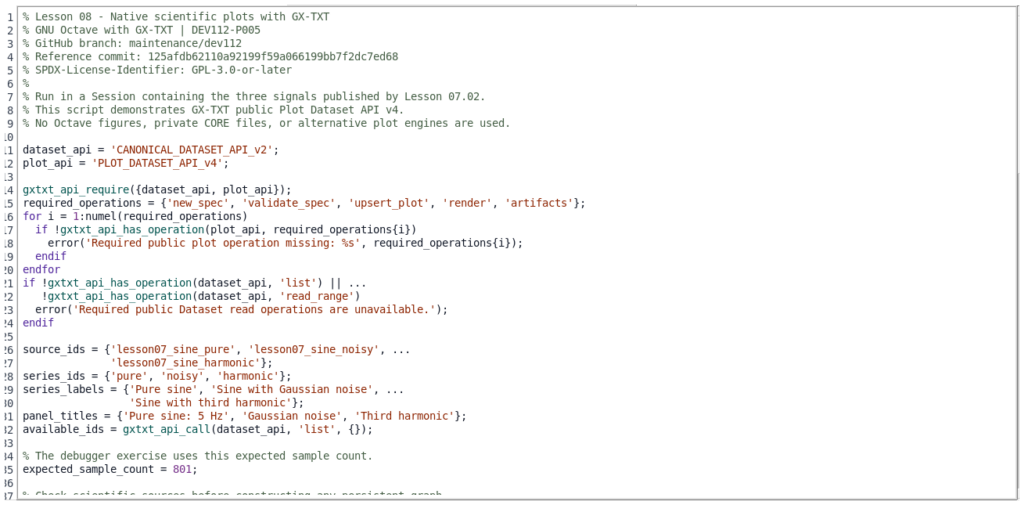
% The debugger exercise uses this expected sample count.
expected_sample_count = 800; % INTENTIONAL BUG: the source has 801 samples.
The same script then reads the actual canonical data and compares the observed sample count with the declared value:
block = gxtxt_api_call(dataset_api, 'read_range', ...
                       {source_ids{i}, {'time_s', 'voltage_v'}, 0, 801});

time_s = block.time_s.values(:);
voltage_v = block.voltage_v.values(:);
actual_sample_count = numel(time_s);

if actual_sample_count != expected_sample_count
  error('Expected %d samples but found %d in %s.', ...
        expected_sample_count, actual_sample_count, source_ids{i});
endif
Octave concepts
numel(time_s) returns the total number of elements in the vector. The operator != means “not equal to,” while the if ... endif statement executes its body only when the condition is true. You encountered these language constructs in the first lessons; here we use them to check the correctness of data read from the framework.
Notice that the script reads the actual Dataset: it does not manufacture a value just to trigger an error.
The expression block.time_s.values(:) extracts the variable values and arranges them into a column vector; source_ids{i} selects the Dataset ID from a cell array. In the call read_range, the value 0 instead identifies the first Dataset row: GX-TXT read indices start at zero, whereas ordinary Octave indices start at one, as explained in Lesson 06.
What the debugger shows
A debugger lets you pause a script at a chosen point and inspect its state during execution. A breakpoint is a stopping point, not a change to the calculation. Once it is reached, we can distinguish what the script expected from what its instructions actually produced.
| Tool | What it displays | Why we need it |
|---|---|---|
| Breakpoint | The line at which execution should pause. | Pause before the check that could raise the error. |
| Variables / Locals | The values of variables in the current observed context. | Compare 800 and 801 directly, rather than inferring the difference only from the final error message. |
| Call Stack | The sequence of calls that led to the current execution point. | Identify the function and source line where execution is paused. |
| Continue and Step Over | Resume execution or step past one instruction. | Observe when the incorrect condition is evaluated. |
The debugger operates on the script revision saved and registered in the Session. Therefore, you must save your changes before starting a Debug Job: the Job must execute an identifiable version of the code.
Setting a real breakpoint
In the source editor, navigate to line 49, which contains the comparison. Open Run > Debug Session script…. Select the line and click Breakpoint.
Click Start Debug. GX-TXT starts a managed debugging Job, pauses execution at the breakpoint, and displays the registered version of the script used by that Job.
In Stack and variables, inspect these two local variables:
| Local variable | Observed value |
|---|---|
actual_sample_count | 801 |
expected_sample_count | 800 |
The difference reveals the defect before the exception is raised.

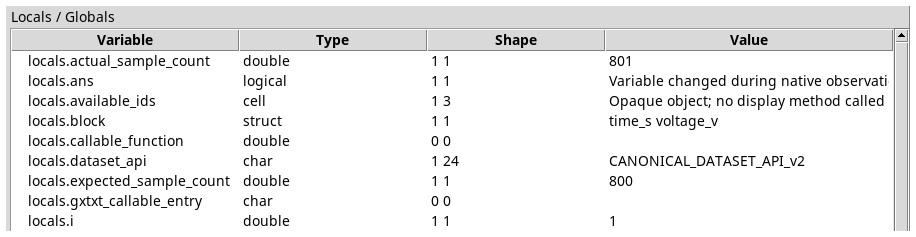
Click Continue. GNU Octave evaluates the condition, which is true, and raises the following message:
Expected 800 samples but found 801 in lesson07_sine_pure.The Job ends with status FAILED: this is the expected result of this intentionally incorrect exercise. This is not a GX-TXT defect. Execution stops before either scientific graph is created.

Debugger clarification: after an error, a snapshot labeled “last paused” shows values observed at the last pause, not live variables from a function whose execution has already unwound.
4. Correcting the error
Open the corrected script L08_02_Native_Plots_Correct.m. The scientific procedure is identical, but the expected sample count is now correct:
expected_sample_count = 801;We use two separate registered scripts: one containing the error and one corrected. This lets us compare the two Jobs and demonstrates an important principle: the debugger refers to the script revision that was actually executed, not to later changes made in the editor.
5. Public GX-TXT APIs used in this lesson
A scientific script must interact through the public Script Bridge surface, without directly calling Tcl procedures, reading private Session files, or invoking internal rendering routines.
5.1 Declaring dependencies
dataset_api = 'CANONICAL_DATASET_API_v2';
plot_api = 'PLOT_DATASET_API_v4';

gxtxt_api_require({dataset_api, plot_api});
gxtxt_api_require() checks the availability of the requested public APIs in the managed script context. Its argument is a cell array, an Octave data structure containing API identifiers.
The next check is more specific:
required_operations = {'new_spec', 'validate_spec', ...
                       'upsert_plot', 'render', 'artifacts'};
for i = 1:numel(required_operations)
  if !gxtxt_api_has_operation(plot_api, required_operations{i})
    error('Required public plot operation missing: %s', ...
          required_operations{i});
  endif
endfor
gxtxt_api_has_operation(api_id, operation) verifies that a particular Script Bridge operation is actually registered. Knowing an API family name does not automatically authorize access to arbitrary internal procedures.
For a more detailed description of the available operations, use gxtxt_api_describe('PLOT_DATASET_API_v4') in a managed script, or open the GX-TXTAPI Browser . Operation descriptors can document argument and result contracts.
5.2 Consulting a canonical Dataset
available_ids = gxtxt_api_call(dataset_api, 'list', {});
block = gxtxt_api_call(dataset_api, 'read_range', ...
                      {'lesson07_sine_pure', {'time_s','voltage_v'}, ...
                       0, 801});
CANONICAL_DATASET_API_v2 / list returns the IDs of Datasets registered in the current Session.
CANONICAL_DATASET_API_v2 / read_range reads a bounded number of rows using stable Variable IDs. The parameters are:
- The Dataset ID.
- A cell array containing the IDs of the variables to read.
- The starting row index, beginning at zero.
- The requested number of rows.
The result contains a structure for each selected variable, including its values. Reading does not depend on a CSV file path or the physical order of columns.
5.3 Defining a PlotSpec instead of drawing a figure
overlay = gxtxt_api_call(plot_api, 'new_spec', ...
                         {'plot.dataset.xy', ...
                          'Lesson 08: signal comparison'});
PLOT_DATASET_API_v4 / new_spec creates an initial declarative specification. The graph type plot.dataset.xy identifies a Cartesian X/Y representation.
The PlotSpec describes panels, axes, series, and presentation options. Dataset content remains the authoritative scientific source, independently of how it is plotted.
What a PlotSpec contains
A PlotSpec is a structured description of how to display scientific data that already exists. It does not necessarily contain the curve samples: it states which Dataset and Variable IDs to use and how to arrange them. The new_spec operation returns an Octave structure that we can complete before requesting rendering.
| Element | Role in the representation |
|---|---|
title | The overall graph title. |
panels | A cell array containing the graph panels. |
axes | Axis labels and scales for each panel. |
series | The curves in a panel, including references to their Datasets. |
multi_panel | Enables vertically stacked panels sharing the X axis. |
This model is declarative: we prepare and validate a data structure, then let GX-TXT generate the graph. This differs from drawing a curve by issuing a sequence of direct graphics commands to Octave.
Do not confuse the API version with the specification version: Plot Dataset API v4 identifies the version of the public service used by the script, while PlotSpec v2 identifies the format of the structure describing the graph. These are separate and compatible versioning schemes.
5.4 The graph lifecycle
| Public operation | Purpose |
|---|---|
new_spec | Create a valid initial PlotSpec structure |
validate_spec | Reject invalid or inconsistent graph specifications |
upsert_plot | Create or update a persistent script-owned graph or variant using a stable producer key |
render | Render the persistent graph through the framework |
artifacts | Inspect public paths and metadata for generated artifacts |
All these calls use the same Script Bridge entry point:
result = gxtxt_api_call(plot_api, operation, arguments);The arguments parameter is a cell array of positional arguments. The Script Bridge maps the public operation to the framework provider, checks its contract, and returns a structured result.
Persistent graph, variant, and stable key
Lesson 06 already used Plot Dataset API v4 to create a bar chart. Here we examine its behavior in more detail: validate_spec checks that the specification is consistent, whereas upsert_plot registers the representation using a stable key owned by the producing script. If the same script runs again in the same Session, that key allows the associated representation to be updated instead of automatically creating a new one on every run.
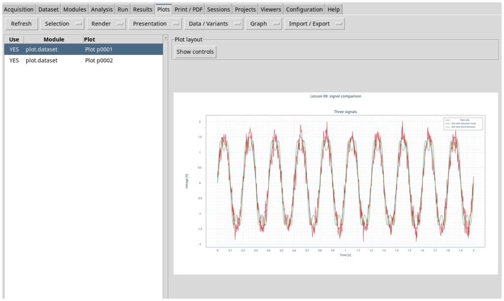
The result of upsert_plot is a graph reference (used by the subsequent render and artifactscalls). It must not be confused with the dataset_id: the former identifies a representation, while the latter identifies its scientific data source. Variants therefore allow different views of the same data to be retained. The identifiers p0001 and p0002 mentioned below were assigned in the exercise Session; they may differ in another Session.
6. First graph: three overlaid curves
For each curve, we describe both its scientific identity and how it should be displayed:
p.series{i} = struct( ...
    'id', series_ids{i}, ...
    'label', series_labels{i}, ...
    'dataset_id', source_ids{i}, ...
    'x_variable_id', 'time_s', ...
    'y_variable_id', 'voltage_v', ...
    'axis', 'left', ...
    'kind', 'line');
The dataset_id and the two variable_id values are not merely labels. They refer to resources already published in the current GX-TXT Session.
The axis field selects the left Y axis, and kind='line' requests a line representation. The label field defines the text displayed in the legend.
In Octave, struct(...) creates the description of one series, while p.series{i} stores it at position i of a cell array. Curly braces {} access the contents of cells, whereas dot notation accesses structure fields. These forms of access, introduced in Lessons 05 and 07, work together here.
It is useful to distinguish three identities: id is the identifier of the series within the graph; dataset_id identifies the source Dataset; x_variable_id and y_variable_id select the two variables to plot. Finally, axis = left binds the series to the left Y axis, while the axes.y_left field configures that axis’s properties.
The script builds three such structures in one panel, configures axis labels, validates the PlotSpec, then registers and renders it:
if !gxtxt_api_call(plot_api, 'validate_spec', {overlay})
  error('The three-trace overlay PlotSpec failed validation.');
endif

ref_overlay = gxtxt_api_call(plot_api, 'upsert_plot', ...
                             {'lesson08_signal_overlay', overlay});
gxtxt_api_call(plot_api, 'render', {ref_overlay});
artifact_overlay = gxtxt_api_call(plot_api, 'artifacts', {ref_overlay});
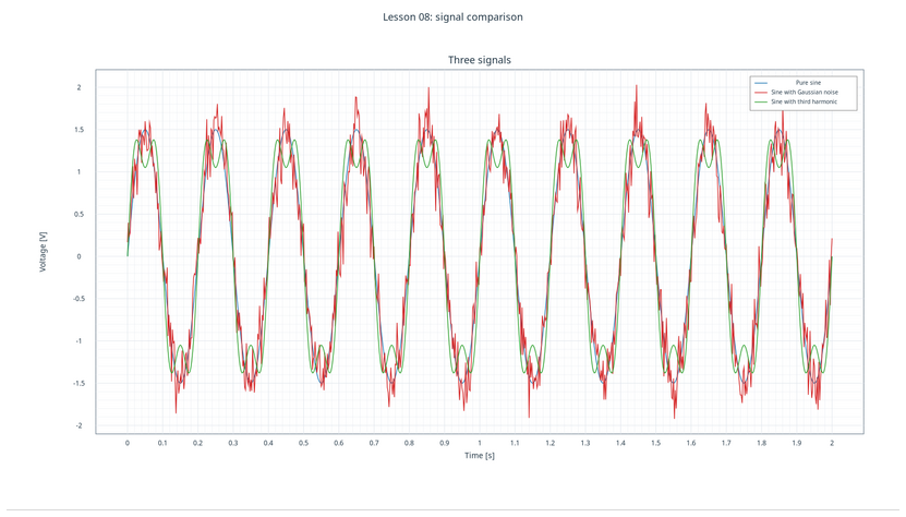
The result, GX-TXT graph variant p0001, displays all three 5 Hz signals together. The noisy curve is recognizable from its irregular departures from the ideal sine wave, while the third harmonic changes the waveform shape.
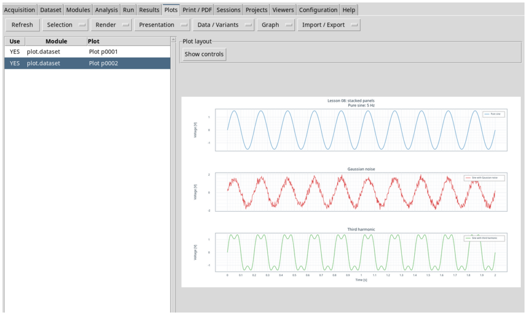
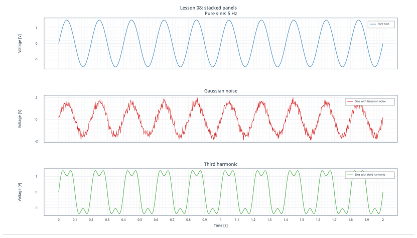
7. Second graph: three vertically stacked panels
Overlapping curves can sometimes conceal important differences. The PlotSpec v2, available through Plot Dataset API v4, also supports vertically stacked panels sharing the X axis.
stacked = gxtxt_api_call(plot_api, 'new_spec', ...
                         {'plot.dataset.xy', ...
                          'Lesson 08: stacked panels'});
stacked.multi_panel = 1;
stacked.panels = cell(1, numel(source_ids));
A cell array created using cellcan hold multiple structures describing the panels. A for loop creates one for each scientific signal:
With cell(1, numel(source_ids)) we allocate space for each of the three panels. Preallocation makes the intended structure size explicit before the forloop fills it, a technique already encountered in Lesson 07. Each panel has its own id, a title, and a list of series.
for i = 1:numel(source_ids)
  panel = struct();
  panel.id = series_ids{i};
  panel.title = panel_titles{i};
  panel.axes = struct( ...
      'x', struct('label', 'Time [s]', 'scale', 'linear'), ...
      'y_left', struct('label', 'Voltage [V]', 'scale', 'linear'));
  panel.annotations = {};
  panel.series = {p.series{i}};
  stacked.panels{i} = panel;
endfor
The essential distinction is that we do not publish the data again. The second PlotSpec describes a different representation of the same Dataset/Variable IDs already in the Session.
In the panel.axesstructure, the x and y_left fields themselves contain structures with label and scale: these are nested structures. Assigning panel.series = {p.series{i}} places a single curve in the current panel. Setting stacked.multi_panel = 1makes GX-TXT arrange the panels vertically: the time axis X is shared, while each panel can have its own Y representation.
We validate and render it as in the first case. The resulting independent graph is variant p0002.
Which representation should you choose?
An overlay is useful when we want to compare the three signals at the same instant, directly observing their deviations from the ideal sine wave. Separate panels are easier to read when curves cross or noise obscures differences in shape. Neither representation changes Dataset values: only the way the data is viewed changes.
8. Exercises
- Change the global title of the overlaid graph and observe how the update affects the same persistent graph variant.
- Change the legend label of one curve; verify that the source Dataset ID and Variable IDs have not changed.
- Compare the overlay with the three-panel representation. Which makes Gaussian noise easier to recognize? Which highlights the third harmonic more clearly?
- Set a breakpoint on the instruction
actual_sample_count = numel(time_s);and perform a Step Over. Observe how the variable’s value changes. - Restore the intentional error by setting the value to 800, run only the debugging exercise in a test Session, then correct it again.
9. Common errors
“Missing Dataset” means that Lesson 07.02 has not been run in the current Session, or that the source Dataset IDs differ. Do not silently replace a missing scientific Dataset with a numeric array created in the script.
“Missing public plot operation” means that the required Script Bridge declaration or its module is not available in the active framework and script context.
“Expected 800 samples but found 801” is the error deliberately introduced into the first version. The intended fix is to set the expected sample count to 801.
“Invalid Variable ID” means that a binding does not match a variable descriptor actually present in the Session Dataset. Consult the canonical schema instead of guessing IDs from column positions.
10. Lesson resources
L08_00_Prerequisite_L07_Signals.m— prerequisite script equivalent to Lesson 07.02.L08_01_Debug_Exercise_Buggy.m— script containing the intentional error.L08_02_Native_Plots_Correct.m— corrected and verified implementation based on public APIs.
The lesson combines two levels of the exercise: in GNU Octave, we organize structures, check data, and construct graph specifications; through the public APIs, GX-TXT consults canonical Datasets and retains persistent graphical representations in the Session.
Public source references
- GX-TXT GitHub repository, maintenance/dev112
- Plot Dataset API v4
- Plot Dataset API v2 — PlotSpec and panel layout
- GNU Octave Script Workspace
Validation scope: this lesson was verified on DEV112-P005. Later revisions published on GitHub may change elements of the interface or introduce new public operations, so the exact reference commit is provided.
Other steps of this project
- Lesson 01 — Your First GNU Octave Script in GX-TXT
- Lesson 02 — Variables, Data Types and Operators in GNU Octave with GX-TXT
- Lesson 03 — Vectors and Matrices in GNU Octave with GX-TXT: Temperature Measurement Analysis
- Lesson 04 — Conditions, Loops, and Functions. Simulating Newton’s Law of Cooling
- Lesson 05: Scientific Datasets and Variable IDs
- Lesson 06 — Selecting and Reading Experimental Data with GNU Octave and GX-TXT