

GNU Octave and GX-TXT: Complex Arithmetic and Bode Diagrams with Numeric API v1
In Lesson 15 of the GNU Octave with GX-TXT course, we computed the frequency response of a series RLC circuit using mainly the language’s native functions. The framework’s public APIs were used to read and publish Datasets and to visualize them. This in-depth article revisits the same physical model, but focuses on the public numerical operations of the math.numeric module: how to invoke them, what they return, which errors they check, and why they are not always interchangeable with Octave functions or the Script Bridge.
1. What Does a Numeric API Add to Native Octave Functions?
GNU Octave already provides abs(z), angle(z), log10(x), and complex-number division. GX-TXT does not replace these capabilities: NUMERIC_API_v1 exposes a public mathematical service with explicit operation names, arguments, and results. Its purpose is to let framework components share documented computations and checks without using private commands or manipulating internal files.
This does not mean that the API necessarily achieves greater numerical precision than Octave. Its main value lies in its contract: array shapes, policies for nonfinite values, separation of complex components, result structures, and error handling. Even when we use the framework, Octave remains the language in which we build the experiment, select samples, and perform independent checks.
This article connects with earlier published lessons: Lesson 02 — Variables and Operators, Lesson 07 — Datasets and the Numeric API, Lesson 13 — FFT and Phase, and Lesson 15 — RLC Circuits and Bode Diagrams.
2. Framework Version and the Boundary Between Two Public Interfaces
| Reference | Version used |
|---|---|
| GX-TXT framework | 0.9.8.10-dev-112, Release 2, P011 |
| GitHub release | v0.9.8.10-dev-112-r2-p011 |
| Source commit | 9f79a30661d6a3fe4a05d723be66aabd06ef2ebe |
| Scientific module | math.numeric, NUMERIC_API_v1 |
| Language and runtime | GNU Octave 9.4.0 |
| Code license | GPL-3.0-or-later |
It is essential to distinguish two access paths.
- The public Octave binding of the Numeric module is invoked using
gxtxt_numeric_v1('operation', ...). It accepts the arrays specified by the module contract and returns Octave structures. - The managed Octave Script Bridge is invoked using
gxtxt_api_call('NUMERIC_API_v1','operation',{...})and requires the operation to be registered in the Script Bridge catalog. For some real-array operations, operands are descriptors containingkindandvalue.
In commit P011, array_unary and array_binary are exposed through both paths, but complex_unary, complex_binary and unwrap do not appear as operations with those names in the inspected Script Bridge binding. They are available through the Numeric module’s direct Octave interface. It would therefore be incorrect to automatically turn a call to gxtxt_numeric_v1('complex_binary',...) into gxtxt_api_call('NUMERIC_API_v1','complex_binary',...).
The complete experiment attached to this article uses the direct public Octave interface. It was executed on an isolated P011 framework copy and also using the unmodified binding file retrieved from the stated GitHub commit. We do not present it as a Script Workspace Job validated with these complex operations. Reading and publishing Datasets remain the subjects of earlier lessons.
3. The RLC Circuit: From Physical Laws to Complex Numbers
Consider a resistor \(R=20\ \Omega\), an inductor \(L=10\ \mathrm{mH}=0.010\ \mathrm{H}\), and a capacitor \(C=1\ \mu\mathrm{F}=10^{-6}\ \mathrm{F}\), connected in series. We apply a sinusoidal voltage and measure the output across the resistor, using a consistent input/output polarity convention.
With angular frequency \(\omega=2\pi f\), the impedances are:
\[Z_R=R,\qquad Z_L=j\omega L,\qquad Z_C=\frac{1}{j\omega C}.\]
In sinusoidal steady state, the same current passes through all components. Applying Kirchhoff’s voltage law and dividing the resistor-voltage phasor by the input-voltage phasor gives:
\[\begin{aligned}H(j\omega)&=\frac{\widehat V_R}{\widehat V_{\mathrm{in}}}=\frac{R}{R+jX(\omega)},\\ X(\omega)&=\omega L-\frac{1}{\omega C}.\end{aligned}\]
The complex transfer function contains two pieces of information: \(|H|\) is the voltage-amplitude ratio, and \(\arg H\) is the output phase relative to the input. Changing the output terminals would change the function. The model is ideal: it includes neither parasitic losses nor component uncertainties.
4. Result Structures: values, real and imaginary
A public operation does not always return a simple vector: its result is a structure with documented fields. Real-array operations generally return values; a complex result from complex_binary contains real and imaginary.
| Public operation | Purpose | Result fields |
|---|---|---|
array_binary('multiply',a,b) | Element-wise real multiplication | .values |
array_binary('divide',a,b) | Real division | .values |
array_binary('subtract',a,b) | Real subtraction | .values |
array_unary('log10',x) | Base-ten real logarithm | .values |
complex_binary('divide',reA,imA,reB,imB) | Complex division | .real, .imaginary |
complex_unary('magnitude',re,im) | Complex magnitude | .values |
complex_unary('phase_rad',re,im) | Phase in radians | .values |
complex_unary('phase_deg',re,im) | Phase in degrees | .values |
unwrap(phase, options) | Remove full-period discontinuities | .values, .period |
For example, transfer.imaginary is correct, whereas transfer.imag is not a field returned by complex_binary. The separate-components representation (split-complex) is a data contract, not a mathematical approximation: conceptually, we can always reconstruct \(z=\mathrm{real}+j\,\mathrm{imaginary}\).
The elementary operations explicitly handle shape compatibility. A scalar can be expanded to work with a vector; two nonscalar arrays must have compatible shapes. By default, nonfinite data and results outside the real domain are rejected. These APIs do not automatically convert mH to H or radians to degrees unless the appropriate operation is requested: physical units must be consistent before the calculation.
5. Experiment: Constructing Reactance with array_binary
We generate a logarithmic vector of 401 frequencies and insert the exact theoretical resonance frequency to obtain 402 samples. Octave’s logspace and sort build the vector; GX-TXT handles the numerical operations on angular frequency and reactance.
R_ohm = 20;
L_h = 10e-3;
C_f = 1e-6;
f0_hz = 1/(2*pi*sqrt(L_h*C_f));
frequency_hz = sort([logspace(2,4.5,401)'; f0_hz]);

omega_result = gxtxt_numeric_v1('array_binary', ...
  'multiply',2*pi,frequency_hz);
omega = omega_result.values;

XL = gxtxt_numeric_v1('array_binary','multiply',L_h,omega);
omega_C = gxtxt_numeric_v1('array_binary','multiply',C_f,omega);
XC_mag = gxtxt_numeric_v1('array_binary','divide',1,omega_C.values);
reactance = gxtxt_numeric_v1('array_binary', ...
  'subtract',XL.values,XC_mag.values);
X_ohm = reactance.values;
The operations directly implement \(\omega=2\pi f\), \(X_L=\omega L\), \(|X_C|=1/(\omega C)\) and \(X=X_L-|X_C|\). Since the capacitor expression involves division by \(\omega\), our grid does not contain \(f=0\). The sign of \(X\) indicates whether capacitive (negative) or inductive (positive) behavior dominates.
6. complex_binary: Dividing Complex Impedances
We now compute the transfer function \(H=R/(R+jX)\). The complex_binary contract accepts four arrays representing the real and imaginary parts of the two operands, together with the requested operation name:
denominator_real = R_ohm*ones(size(X_ohm));
transfer = gxtxt_numeric_v1('complex_binary','divide', ...
  R_ohm,0,denominator_real,X_ohm);
The numerator has real part \(R\) and zero imaginary part. The denominator has real part \(R\) and imaginary part \(X\). We can understand the result by hand: taking \(R=20\ \Omega\) and \(X=10\ \Omega\),
\[\frac{20}{20+j10}=\frac{20(20-j10)}{20^2+10^2}=0.8-j0.4.\]
Keeping only the real number 0.8 is insufficient: the imaginary component −0.4 is necessary to reconstruct the magnitude (approximately 0.8944) and the output phase lag.
7. complex_unary, Decibels and unwrap
At every frequency, we request two physical projections of the same complex function: its magnitude \(|H|\) and phase \(\varphi=\arg H\).
magnitude = gxtxt_numeric_v1('complex_unary','magnitude', ...
  transfer.real,transfer.imaginary);
phase_degrees = gxtxt_numeric_v1('complex_unary','phase_deg', ...
  transfer.real,transfer.imaginary);

log_magnitude = gxtxt_numeric_v1('array_unary','log10', ...
  magnitude.values);
decibels = gxtxt_numeric_v1('array_binary','multiply', ...
  20,log_magnitude.values);

gain_db = decibels.values;
phase_deg = phase_degrees.values;
The gain of the Bode diagram is computed as
\[G_{\mathrm{dB}}(f)=20\log_{10}|H(j2\pi f)|.\]
The coefficient 20 is used because we compare voltage amplitudes, not powers directly. A negative dB value indicates attenuation, not negative voltage. The magnitude plot uses a logarithmic frequency X-axis in Hz and a numerically linear Y-axis in dB.
Phase is the phase difference between output and input. The phase_deg operation returns it directly in degrees. To understand unwrap as well, we request the phase separately in radians:
phase_radians = gxtxt_numeric_v1('complex_unary','phase_rad', ...
  transfer.real,transfer.imaginary);
unwrapped = gxtxt_numeric_v1('unwrap',phase_radians.values, ...
  struct('period',2*pi));
phase_deg_check = unwrapped.values*180/pi;
unwrap corrects possible jumps of one full period in the angular sequence. It does not convert units: the factor \(180/\pi\) is still needed. In our ideal RLC circuit, phase remains between approximately +90° and −90° and does not cross a 360° discontinuity; this operation illustrates a general capability. If phase were already in degrees, the consistent period would be 360, not \(2\pi\).
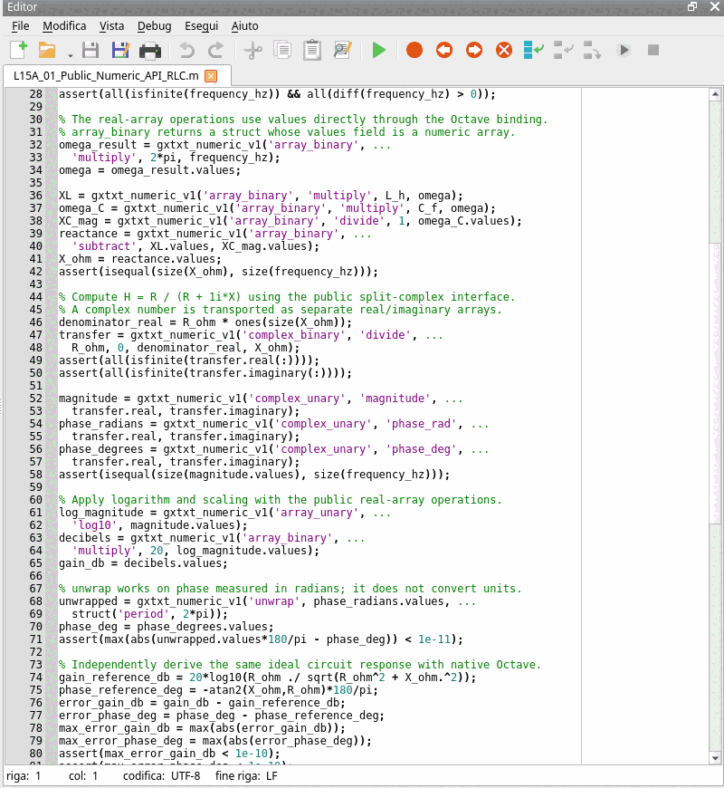
8. Independent Validation and Results on P011
The same physical solution can be derived without performing a division of complex arrays:
\[|H|=\frac{R}{\sqrt{R^2+X^2}},\qquad \varphi=-\operatorname{atan2}(X,R).\]
We use these formulas with native Octave functions as an independent reference, not as a replacement for the Numeric API in the primary calculations:
gain_reference_db = 20*log10(R_ohm ./ ...
  sqrt(R_ohm^2+X_ohm.^2));
phase_reference_deg = -atan2(X_ohm,R_ohm)*180/pi;

max_error_gain_db = max(abs(gain_db-gain_reference_db));
max_error_phase_deg = max(abs(phase_deg-phase_reference_deg));
assert(max_error_gain_db < 1e-10);
assert(max_error_phase_deg < 1e-10);
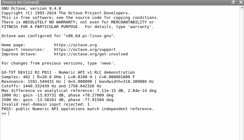
Results obtained with the public P011 binding, also confirmed using the exact GitHub source file:
| Result | Value |
|---|---|
| Samples | 402 |
| Resonance frequency | 1591.549431 Hz |
| Quality factor \(Q\) | 5.000000 |
| Lower half-power frequency | 1440.332439 Hz |
| Upper half-power frequency | 1758.642326 Hz |
| Bandwidth | 318.309886 Hz |
| Maximum gain difference | \(7.11\times10^{-15}\) dB |
| Maximum phase difference | \(2.84\times10^{-14}\) degrees |
As an additional physical spot check, at 1000 Hz we calculated \(-13.83732\ \mathrm{dB}\) and \(+78.27009^\circ\); at 2500 Hz, \(-13.58261\ \mathrm{dB}\) and \(-77.91584^\circ\). Phase changes sign at resonance. Agreement between the methods is consistent with double-precision rounding: it does not demonstrate fourteen-digit instrumental accuracy or quantify the tolerances and noise of real components.
9. An Intentional Error: Real-Domain Calculations Must Not Silently Become Complex
The array_unary API operates on real arrays. Asking for the square root of a negative real number should be rejected. The script explicitly performs this test:
invalid_input_rejected = false;
try
  gxtxt_numeric_v1('array_unary','sqrt',[-4;1]);
catch
  invalid_input_rejected = true;
end_try_catch
assert(invalid_input_rejected);
Rejection is the expected result. Here we catch the exception solely to verify the contract; in an ordinary calculation, we should not hide the error and continue with scientifically invalid data. Likewise, we must check zero denominators, nonfinite values, incompatible shapes, units and sample alignment.
10. How Calls Differ in the Octave Script Workspace
In a GX-TXT managed Job, the public access path is the Script Bridge, which uses a different argument structure. Here we show an operation actually declared by the P011 Bridge binding: multiplication of a real vector by a scalar.
gxtxt_api_require({'NUMERIC_API_v1'});
assert(gxtxt_api_has_operation('NUMERIC_API_v1','array_binary'));

a = struct('kind','vector','value',[1;2;3]);
b = struct('kind','scalar','value',4);
result = gxtxt_api_call('NUMERIC_API_v1', ...
  'array_binary',{'multiply',a,b});
assert(isequal(result.values,[4;8;12]));
Curly braces create a cell array of positional arguments. The kind field describes a scalar or vector, while value contains its data. With the direct binding, the same action is expressed as gxtxt_numeric_v1('array_binary','multiply',[1;2;3],4), without operand descriptors. These are two different contracts.
This snippet illustrates the documented Script Bridge contract, while the complete attached script was executed through the direct Octave binding. We do not claim a separate P011 Session test for the Bridge snippet. To use complex_binary and complex_unary in a Bridge Job, a registered public capability must expose them; private CORE procedures must not be substituted.
11. Reproducing the Experiment and Exercises
To execute the experiment, you need GNU Octave and the public Numeric module from P011, with the gxtxt_numeric_v1 binding available on the Octave API path declared by the module. Check with exist('gxtxt_numeric_v1','file') and which('gxtxt_numeric_v1'). There is no need to open Dataset files, modify the CORE or configure shortcuts to private framework directories.
The complete L15A_01_Public_Numeric_API_RLC.m script includes the formulas, checks, invalid-input rejection and printed results. It ends with PASS: public Numeric API operations match independent reference. This article focuses on numerical APIs, so the script does not publish Datasets or create persistent plots: those operations are documented elsewhere in the course, using DATASET_PUBLICATION_API_v2 and PLOT_DATASET_API_v4.
To check your understanding, try doubling \(R\) and predicting how \(Q\) and bandwidth change; replacing phase_deg with phase_rad and converting correctly; forcing a zero denominator and observing the rejected calculation; and introducing incompatible complex-array sizes to explain why element-wise operations cannot combine them.
12. Public Source References
- NUMERIC_API_v1 —
math.numericmodule contract - Public Octave binding
gxtxt_numeric_v1.m math.numericScript Bridge binding- OCTAVE_SCRIPT_BRIDGE_API_v1
The purpose of this in-depth article is to learn how to separate the numerical contract from the physical problem and the execution mechanism. When the experiment is reproducible, we know not only that the result is correct, but also which APIs produced it and which conditions limit its validity.
Complete Downloadable Script
The full source is included in the expandable section below. Code comments and headers are in English; license: GPL-3.0-or-later.
Complete GNU Octave script — L15A_01_Public_Numeric_API_RLC.m
% L15A_01_Public_Numeric_API_RLC.m
% Educational deep dive into GX-TXT Numeric API v1.
% Framework reference: GX-TXT DEV112 R2 P011.
% GitHub commit: 9f79a30661d6a3fe4a05d723be66aabd06ef2ebe
% SPDX-License-Identifier: GPL-3.0-or-later
%
% Run in a GNU Octave module context that exposes the public math.numeric
% binding gxtxt_numeric_v1 on Octave's documented module API path.
% No private CORE functions, data files, or storage providers are accessed.
%
% This script tests the public Octave Numeric binding. It does not claim
% that complex_unary/complex_binary are exposed by the Script Bridge.

if exist('gxtxt_numeric_v1','file') != 2
  error(['Missing gxtxt_numeric_v1 public Octave binding. ', ...
         'Enable the registered math.numeric module API path.']);
endif

R_ohm = 20;
L_h = 10e-3;
C_f = 1e-6;
f0_hz = 1/(2*pi*sqrt(L_h*C_f));
Q_ideal = sqrt(L_h/C_f)/R_ohm;

% Keep one sample at the exact analytical resonance.
frequency_hz = sort([logspace(2, 4.5, 401)'; f0_hz]);
assert(numel(frequency_hz) == 402);
assert(all(isfinite(frequency_hz)) && all(diff(frequency_hz) > 0));

% The real-array operations use values directly through the Octave binding.
% array_binary returns a struct whose values field is a numeric array.
omega_result = gxtxt_numeric_v1('array_binary', ...
  'multiply', 2*pi, frequency_hz);
omega = omega_result.values;

XL = gxtxt_numeric_v1('array_binary', 'multiply', L_h, omega);
omega_C = gxtxt_numeric_v1('array_binary', 'multiply', C_f, omega);
XC_mag = gxtxt_numeric_v1('array_binary', 'divide', 1, omega_C.values);
reactance = gxtxt_numeric_v1('array_binary', ...
  'subtract', XL.values, XC_mag.values);
X_ohm = reactance.values;
assert(isequal(size(X_ohm), size(frequency_hz)));

% Compute H = R / (R + 1i*X) using the public split-complex interface.
% A complex number is transported as separate real/imaginary arrays.
denominator_real = R_ohm * ones(size(X_ohm));
transfer = gxtxt_numeric_v1('complex_binary', 'divide', ...
  R_ohm, 0, denominator_real, X_ohm);
assert(all(isfinite(transfer.real(:))));
assert(all(isfinite(transfer.imaginary(:))));

magnitude = gxtxt_numeric_v1('complex_unary', 'magnitude', ...
  transfer.real, transfer.imaginary);
phase_radians = gxtxt_numeric_v1('complex_unary', 'phase_rad', ...
  transfer.real, transfer.imaginary);
phase_degrees = gxtxt_numeric_v1('complex_unary', 'phase_deg', ...
  transfer.real, transfer.imaginary);
assert(isequal(size(magnitude.values), size(frequency_hz)));

% Apply logarithm and scaling with the public real-array operations.
log_magnitude = gxtxt_numeric_v1('array_unary', ...
  'log10', magnitude.values);
decibels = gxtxt_numeric_v1('array_binary', ...
  'multiply', 20, log_magnitude.values);
gain_db = decibels.values;

% unwrap works on phase measured in radians; it does not convert units.
unwrapped = gxtxt_numeric_v1('unwrap', phase_radians.values, ...
  struct('period', 2*pi));
phase_deg = phase_degrees.values;
assert(max(abs(unwrapped.values*180/pi - phase_deg)) < 1e-11);

% Independently derive the same ideal circuit response with native Octave.
gain_reference_db = 20*log10(R_ohm ./ sqrt(R_ohm^2 + X_ohm.^2));
phase_reference_deg = -atan2(X_ohm,R_ohm)*180/pi;
error_gain_db = gain_db - gain_reference_db;
error_phase_deg = phase_deg - phase_reference_deg;
max_error_gain_db = max(abs(error_gain_db));
max_error_phase_deg = max(abs(error_phase_deg));
assert(max_error_gain_db < 1e-10);
assert(max_error_phase_deg < 1e-10);
assert(all(gain_db <= 1e-10));

% The exact resonance sample must yield 0 dB and 0 degrees.
[~,res_idx] = min(abs(frequency_hz-f0_hz));
assert(abs(frequency_hz(res_idx)-f0_hz) < 1e-9);
assert(abs(gain_db(res_idx)) < 1e-10);
assert(abs(phase_deg(res_idx)) < 1e-10);

omega_1 = (-R_ohm + sqrt(R_ohm^2+4*L_h/C_f))/(2*L_h);
omega_2 = ( R_ohm + sqrt(R_ohm^2+4*L_h/C_f))/(2*L_h);
f1_hz = omega_1/(2*pi);
f2_hz = omega_2/(2*pi);
bandwidth_hz = f2_hz-f1_hz;
assert(abs(Q_ideal-f0_hz/bandwidth_hz) < 1e-10);

% Demonstrate explicit error handling rather than silently hiding it.
invalid_input_rejected = false;
try
  gxtxt_numeric_v1('array_unary','sqrt',[-4;1]);
catch
  invalid_input_rejected = true;
end_try_catch
assert(invalid_input_rejected);

% Print only scientifically relevant measurements and validation facts.
fprintf('GX-TXT DEV112 R2 P011 - Numeric API v1 RLC demonstration\n');
fprintf('Samples: %d | R=%.1f Ohm | L=%.4f H | C=%.9f F\n', ...
  numel(frequency_hz), R_ohm, L_h, C_f);
fprintf('Resonance: %.6f Hz | Q=%.6f | bandwidth=%.6f Hz\n', ...
  f0_hz, Q_ideal, bandwidth_hz);
fprintf('Cutoffs: %.6f Hz and %.6f Hz\n', f1_hz, f2_hz);
fprintf('Max difference vs analytical reference: %.3g dB, %.3g deg\n', ...
  max_error_gain_db, max_error_phase_deg);
for f_sample = [1000, 2500]
  w = 2*pi*f_sample;
  xx = w*L_h-1/(w*C_f);
  hh = R_ohm/(R_ohm+1i*xx);
  fprintf('%g Hz: gain %.5f dB, phase %+.5f deg\n', ...
    f_sample, 20*log10(abs(hh)), angle(hh)*180/pi);
endfor
fprintf('Invalid real-domain input rejected: %d\n',invalid_input_rejected);
fprintf('PASS: public Numeric API operations match independent reference.\n');
From the same category
- Lesson 16 — From UV-Vis Signals to a Kinetic Rate Constant: A Complete Scientific Project with GNU Octave and GX-TXT
- Lesson 15 — RLC Circuits and Bode Diagrams with GNU Octave and GX-TXT
- Lesson 14 – Differential Equations: Chemical Kinetics with GNU Octave and GX-TXT
- Lesson 13 — Spectral Analysis: FFT, Sampling and Windows with GNU Octave and GX-TXT
- Lesson 12 – Linear Algebra: Analyzing a Spectrophotometric Mixture with GNU Octave and GX-TXT
- GX-TXT Temporal Set API: Managing Time Segments and Windows with GNU Octave and Python