

OpenFOAM: heat transfer, natural convection and the Nusselt number
Tenth guide of the Learning OpenFOAM 14 path and the second of the “Turbulence, heat and mass” module of the advanced course, after those on server and transfers, monitoring and convergence, quantitative analysis with ParaView, verification and validation, parameter sweeps, mesh generation, boundary conditions and models, transient simulations and turbulence and RANS models. This one tackles heat transfer and natural convection: energy equation, thermophysical properties, gravity and p_rgh, thermal wall conditions, wall heat flux with wallHeatFlux, Nusselt number and energy balance on the official buoyantCavity case. The deep-dive and practical-tip boxes open with a click: they contain every package script, a reading of the OpenFOAM 14 source code where it decides the result (heat-flux signs, turbulent Prandtl number, wallHeatFlux output), physical estimates for the case, three additional scripts for estimates, power extraction and comparison with the experimental data shipped with the tutorial, and verification procedures.
Series: OpenFOAM on a Linux server, primarily operated from Windows
Edition: OpenFOAM Foundation 14 · ParaView 5.13.2 · October 2026
Level: intermediate · Exercise: heated cavity, parameter study, and thermal energy balance
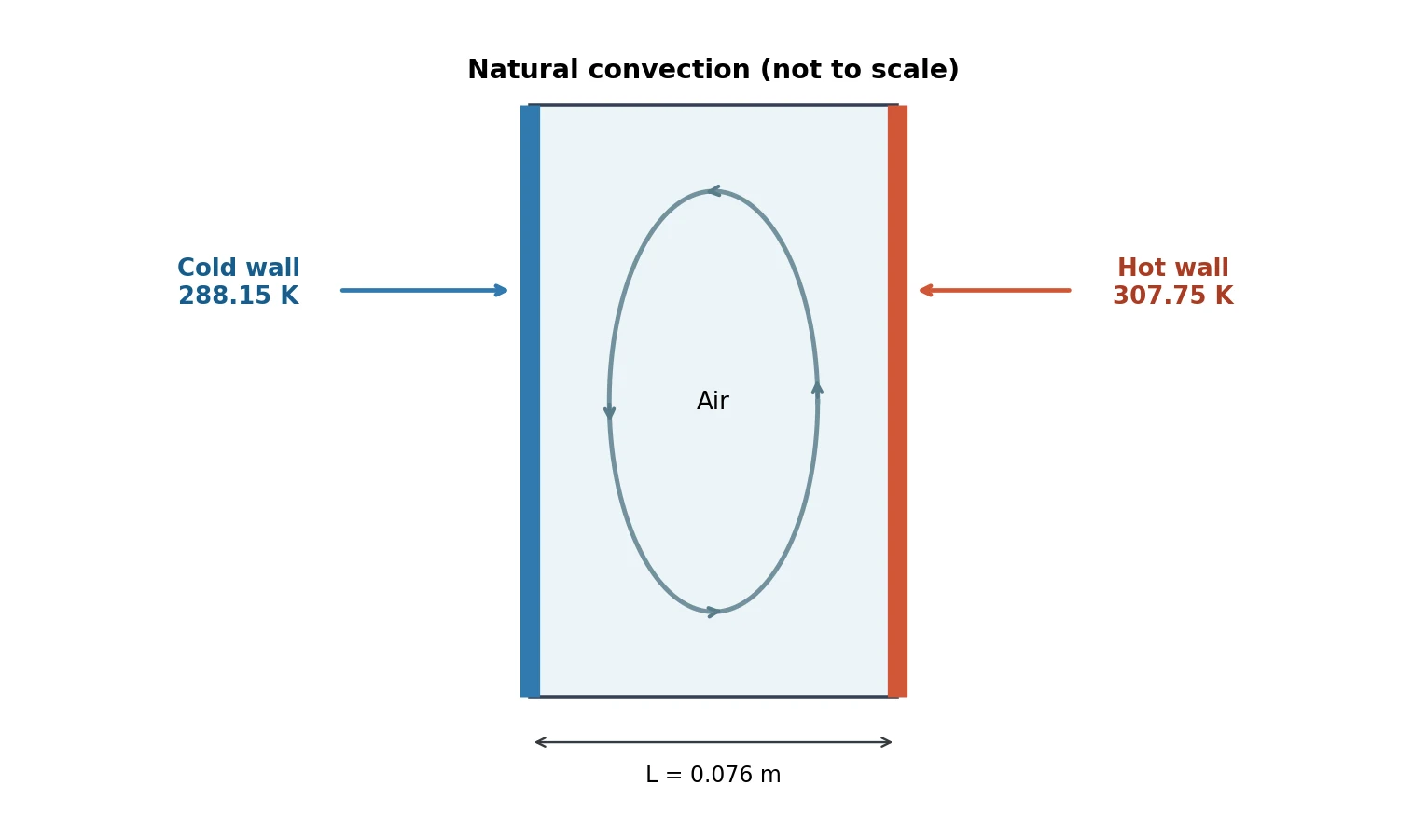
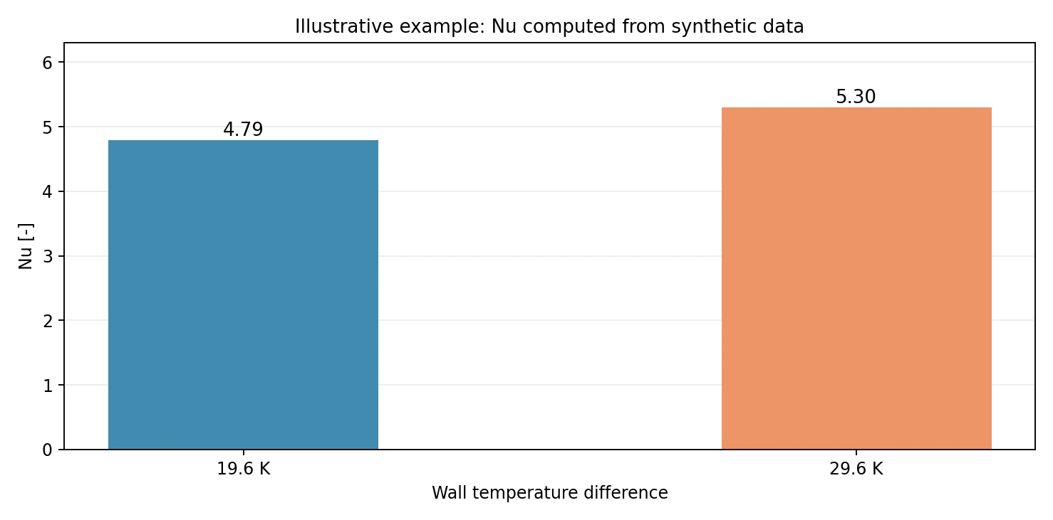
Scope. This guide introduces coupled flow and energy calculations rather than pure heat diffusion. It builds independent copies of the official fluid/buoyantCavity case with ideal-gas air and natural convection. Values in the demonstration charts are synthetic and must not be mistaken for CFD results generated during the preparation of this guide.
1. Objectives and prerequisites
By the end of this guide, readers should be able to identify thermal variables, distinguish isothermal from adiabatic boundaries, configure gravity-driven flow, inspect T, U and p_rgh, obtain wall heat fluxes and interpret a Nusselt number. The solver runs on the Linux server; Windows is used for Notepad++ editing, FileZilla SFTP transfer, and ParaView connected to remote pvserver.
Prerequisites include an understanding of OpenFOAM’s 0/, constant/, and system/ directories; SSH and foamRun; mesh checks, logs and convergence; and introductory thermal fluid mechanics. Visual Studio Code is not required.
Deep dive · The numbers of the case before any computation
With the tutorial data (air as a perfect gas, M = 28.96 g/mol, p = 10⁵ Pa, cp = 1004.4 J/(kg K), μ = 1.831·10⁻⁵ Pa s, Pr = 0.705) and properties evaluated at the mean wall temperature, the script cavity_estimates.py (next box) gives:
| Quantity | ΔT = 19.6 K | ΔT = 29.6 K | Meaning |
|---|---|---|---|
| mean temperature | 297.95 K | 302.95 K | reference for properties |
| density hot / cold wall | 1.132 / 1.209 kg/m³ | 1.096 / 1.209 kg/m³ | perfect gas, p = 10⁵ Pa |
| Δρ/ρ | 6.6 % | 9.8 % | still within the range where Boussinesq would be acceptable |
| RaW = gβΔT W³/(να) | 8.1·10⁵ | 1.2·10⁶ | based on width W = 0.076 m |
| RaH | 1.9·10¹⁰ | 2.8·10¹⁰ | based on height H = 2.18 m: turbulent boundary layers |
| buoyancy velocity √(gβΔT W) | 0.22 m/s | 0.27 m/s | upper scale of the vertical velocity |
| conduction-only power (NuW = 1) | 7.6 W | 11.5 W | physical lower bound |
| NuW from correlation (ERH 1982) | 5.65 | 6.37 | expected order of magnitude |
| estimated power Nu · Qcond | ≈ 43 W | ≈ 73 W | to be compared with wallHeatFlux |
The aspect ratio H/W = 28.7 and RaW of order 10⁶ place the problem within the range of the Elsherbiny, Raithby and Hollands correlation for vertical cavities (5 ≤ H/W ≤ 110, RaW up to about 2·10⁷). The header of the experimental files shipped with the tutorial reports Ra = 8.6·10⁵: the small difference from the computed value comes from the air properties used. The case sheet in the ERCOFTAC database (KBwiki, UFR 4-10) reports for the experiment a mean Nusselt number of 5.85 with ΔT = 19.6 °C (Ra = 0.86·10⁶) and 7.57 with ΔT = 39.9 °C (Ra = 1.43·10⁶): the correlation is within 4 % and, with Nu = 5.85, the expected power is about 44.6 W. If the power computed by OpenFOAM differs from these values by a factor of 2, look for sign, area or convergence errors before any physical interpretation.
Deep dive · Additional script: cavity_estimates.py
Computes properties at the mean value, Rayleigh numbers, conduction-only power, Nusselt number from the correlation and an upper bound of the radiative exchange between two grey parallel plates (box in section 6). It uses only the Python standard library and runs on Windows and Linux:
python cavity_estimates.py
python cavity_estimates.py --Th 317.75
python cavity_estimates.py --emissivity 0.05 0.9
#!/usr/bin/env python3
# SPDX-License-Identifier: GPL-3.0-or-later
"""Order-of-magnitude estimates for the OpenFOAM 14 buoyantCavity case.
Computes ideal-gas properties at the mean temperature, Rayleigh numbers based on
gap width and height, the conduction-only heat rate, the Elsherbiny-Raithby-
Hollands (1982) correlation for vertical cavities and the radiative exchange
between two parallel grey plates. Nothing here is a CFD result: use the numbers
only to judge whether simulated wall powers are plausible.
"""
import argparse
import math
R_UNIVERSAL = 8.314462618 # J/(mol K)
SIGMA = 5.670374419e-8 # W/(m2 K4)
def erh_nusselt(ra, aspect):
"""Elsherbiny, Raithby & Hollands (1982), vertical cavity, isothermal walls.
Stated range: 5 <= H/W <= 110 and Ra_W up to about 2e7. Returns Nu_W.
"""
nu1 = 0.0605 * ra ** (1.0 / 3.0)
nu2 = (1.0 + (0.104 * ra ** 0.293 / (1.0 + (6310.0 / ra) ** 1.36)) ** 3) ** (1.0 / 3.0)
nu3 = 0.242 * (ra / aspect) ** 0.272
return max(nu1, nu2, nu3), (nu1, nu2, nu3)
def main():
p = argparse.ArgumentParser(description=__doc__)
p.add_argument('--Th', type=float, default=307.75, help='hot wall temperature [K]')
p.add_argument('--Tc', type=float, default=288.15, help='cold wall temperature [K]')
p.add_argument('--W', type=float, default=0.076, help='gap width [m]')
p.add_argument('--H', type=float, default=2.18, help='cavity height [m]')
p.add_argument('--D', type=float, default=0.52, help='cavity depth [m]')
p.add_argument('--p', type=float, default=1e5, help='pressure [Pa]')
p.add_argument('--M', type=float, default=28.96, help='molar mass [g/mol]')
p.add_argument('--Cp', type=float, default=1004.4, help='specific heat [J/(kg K)]')
p.add_argument('--mu', type=float, default=1.831e-5, help='dynamic viscosity [Pa s]')
p.add_argument('--Pr', type=float, default=0.705, help='Prandtl number [-]')
p.add_argument('--g', type=float, default=9.81, help='gravity [m/s2]')
p.add_argument('--emissivity', type=float, nargs='*', default=[0.05, 0.1, 0.3, 0.9],
help='wall emissivities for the radiative bound (both walls equal)')
a = p.parse_args()
if not a.Th > a.Tc > 0:
p.error('Expected Th > Tc > 0 K')
dT = a.Th - a.Tc
Tm = 0.5 * (a.Th + a.Tc)
Rs = R_UNIVERSAL / (a.M * 1e-3)
rho_m, rho_h, rho_c = (a.p / (Rs * T) for T in (Tm, a.Th, a.Tc))
k = a.mu * a.Cp / a.Pr
nu = a.mu / rho_m
alpha = k / (rho_m * a.Cp)
beta = 1.0 / Tm
ra_w = a.g * beta * dT * a.W ** 3 / (nu * alpha)
ra_h = ra_w * (a.H / a.W) ** 3
aspect = a.H / a.W
area = a.H * a.D
q_cond = k * dT * area / a.W
nu_erh, parts = erh_nusselt(ra_w, aspect)
u0 = math.sqrt(a.g * beta * dT * a.W)
print('Mean temperature Tm = %.2f K' % Tm)
print('Density hot / mean / cold = %.4f / %.4f / %.4f kg/m3' % (rho_h, rho_m, rho_c))
print('Relative density difference = %.2f %%' % (100 * (rho_c - rho_h) / rho_m))
print('Conductivity k = mu Cp / Pr = %.5f W/(m K)' % k)
print('Kinematic viscosity nu (at Tm) = %.4e m2/s' % nu)
print('Thermal diffusivity alpha (at Tm) = %.4e m2/s' % alpha)
print('Expansion coefficient beta = 1/Tm = %.4e 1/K' % beta)
print('Aspect ratio H/W = %.1f' % aspect)
print('Ra based on W = %.3e' % ra_w)
print('Ra based on H = %.3e' % ra_h)
print('Buoyancy velocity sqrt(g beta dT W) = %.3f m/s' % u0)
print('Wall area H x D = %.4f m2' % area)
print('Conduction-only power (Nu_W = 1) = %.2f W' % q_cond)
print('ERH 1982: Nu1, Nu2, Nu3 = %.2f, %.2f, %.2f' % parts)
print('ERH 1982: Nu_W = max(...) = %.2f -> Q ~ %.1f W' % (nu_erh, nu_erh * q_cond))
if not (5 <= aspect <= 110 and ra_w <= 2e7):
print('WARNING: outside the stated range of the ERH correlation')
q_bb = SIGMA * (a.Th ** 4 - a.Tc ** 4)
for eps in a.emissivity:
if not 0 < eps <= 1:
p.error('emissivity must be in (0, 1]')
q_rad = q_bb / (2.0 / eps - 1.0)
print('Radiation, eps = %.2f: q = %.1f W/m2, Q = %.1f W (infinite parallel plates)' % (eps, q_rad, q_rad * area))
if __name__ == '__main__':
main()The correlation formulas are in the function erh_nusselt: Nu₁ = 0.0605 Ra1/3, Nu₂ = [1 + (0.104 Ra0.293/(1 + (6310/Ra)1.36))³]1/3, Nu₃ = 0.242 (Ra/A)0.272, Nu = max(Nu₁, Nu₂, Nu₃). They are experimental correlations with a typical uncertainty of the order of 10 %: use them to judge plausibility, not to validate.
Practical tip · Define the measurements before launching
Write in a text file in the study folder the quantities you will compare and their exact definition: “Qhot = Q value of the hot patch in the wallHeatFlux file at the last iteration, positive when entering the fluid”, “NuW with L = 0.076 m, k = 0.026086 W/(m K), ΔT = Thot − Tcold”, “convergence: change of Qhot below 0.1 % over the last 100 iterations”. Fixing definitions and criteria before the results prevents choosing afterwards the one that confirms the hypothesis.
2. What changes when thermal effects are included?
An isothermal incompressible simulation is primarily driven by momentum and mass continuity. Heat transfer requires an energy equation, thermophysical properties and suitable boundary conditions for T.
A schematic temperature equation for constant properties and no source is:
ρ cp ( ∂T/∂t + u·∇T ) = ∇·( k ∇T )
This is an explanatory equation, not an exact transcription of the case implementation. The selected OpenFOAM tutorial uses an enthalpy formulation with ideal-gas thermophysical modelling. p_rgh accounts for gravitational hydrostatic effects and should not automatically be treated as absolute gas pressure.
Optional refresher — the three mechanisms. Conduction is energy transfer associated with a temperature gradient; convection is energy transport involving fluid motion; radiation transfers energy electromagnetically and is not enabled in the baseline case. Here, fluid motion is driven by buoyancy due to density differences.
Deep dive · The energy equation OpenFOAM 14 actually solves
In the fluid module (file applications/modules/fluid/thermophysicalPredictor.C in the version 14 source) the unknown is the sensible enthalpy h, not temperature. The assembled equation is, in symbolic form:
ddt(rho, h) + div(phi, h) + ddt(rho, K) + div(phi, K) - dp/dt + divq(h)
    = rho*(U & g) + fvModels sources

K = |U|^2/2            kinetic energy per unit mass
phi                    mass flux on faces [kg/s]
divq(h)                molecular + turbulent heat flux
With thermo hConst the sensible enthalpy is h = cp (T − Tstd), with Tstd = 298.15 K: after each solution T is recovered from h in thermo.correct(). The K terms and pressure work are negligible here (velocities of 0.2 m/s, pressure variations of a few pascals) but they are present: this is why fvSchemes must contain div(phi,K). The rho*(U & g) term only appears when the case has the p_rgh field, i.e. when the buoyancy class is active.
Deep dive · What p_rgh is exactly
The OpenFOAM 14 buoyancy class (src/finiteVolume/cfdTools/general/buoyancy) defines:
p_rgh = p - rho*gh - pRef
gh    = (g & x) - ghRef,      ghRef = -|g| hRef   (hRef optional, default 0)
In the tutorial constant/pRef is 10⁵ Pa and 0/p starts at 10⁵ Pa, so p_rgh starts at zero. With g = (0 −9.81 0) the hydrostatic difference between bottom and top of the cavity is ρ g H ≈ 1.17 · 9.81 · 2.18 ≈ 25 Pa, while the dynamic pressure ½ρU² with U ≈ 0.15 m/s is about 0.013 Pa: three orders of magnitude less. Solving for p_rgh removes the dominant hydrostatic part from the unknown, which would otherwise make small gradients inaccurate. Practical consequence: use p to read physical pressures; p_rgh can be used to compare zones at the same height; never compare p_rgh between cases with different pRef or hRef.
Deep dive · Perfect gas or Boussinesq
The tutorial uses equationOfState perfectGas: ρ = p M/(R T) with the local pressure. The Boussinesq approximation (constant density except in the buoyancy term, ρ ≈ ρ₀[1 − β(T − T₀)]) is considered accurate when βΔT ≲ 0.1. Here βΔT = 0.066 in the baseline and 0.098 in the variant: the hotter case is at the limit. With the perfect gas, β need not be chosen: it is implicit (β = 1/T for a perfect gas). Keep the tutorial model; to study the effect, compare in a new copy with a different density model, documenting it as a model variant.
Practical tip · Check in the log what has been selected
The first lines of logs/foamRun.log report the models actually constructed. Before looking at the results check:
cd "$HOME/OpenFOAM/guide10_thermal_study/baseline_19p6K"
grep -n "Selecting" logs/foamRun.log | head -20
Among others, the heRhoThermo thermodynamics with perfectGas, the kOmegaSST model and the line on the turbulent thermal transport model (box in section 4) must appear. A missing or different line means the case is not the one you think you have.
3. Official buoyantCavity case: geometry and physics
The Foundation tutorial resides at $FOAM_TUTORIALS/fluid/buoyantCavity. It represents a tall three-dimensional air-filled cavity whose lateral walls are held at different temperatures. The original dimensions are 2.180 m high, 0.076 m wide, and 0.520 m deep. Its blockMesh definition contains 35 × 150 × 15 = 78,750 cells. Thermal boundary conditions on the top, bottom, front and back walls are zeroGradient (adiabatic for the selected base model).
| Quantity | Official / baseline | Suggested variant |
|---|---|---|
Hot wall hot | 307.75 K | 317.75 K |
Cold wall cold | 288.15 K | 288.15 K |
| Wall temperature difference | 19.60 K | 29.60 K |
| Gravity | (0 -9.81 0) m/s² | Unchanged |
| Geometry, mesh and model | Unchanged | Unchanged |
The official tutorial refers to the experimental tall-cavity study of Betts and Bokhari (2000). We use the case files supplied with Foundation 14, without claiming that our synthetic figures reproduce the experimental data.
Deep dive · The tutorial mesh up close
From the tutorial system/blockMeshDict (units in mm): x from 0 to 76, y from 0 to 2180, z from −260 to 260; a single block (35 150 15) with simpleGrading (1 1 1). The cold wall is the plane x = 0, the hot wall the plane x = 76 mm; frontAndBack are the planes z = ±260 mm, topAndBottom y = 0 and y = 2180 mm. All patches are of type wall.
| Direction | Cells | Spacing | Comment |
|---|---|---|---|
| x (between thermal walls) | 35 | 2.17 mm | first cell centre 1.09 mm from the wall |
| y (height) | 150 | 14.5 mm | cell aspect ratio Δy/Δx ≈ 6.7 |
| z (depth) | 15 | 34.7 mm | Δz/Δx ≈ 16: very elongated cells |
The experimental data shipped with the tutorial (validation/exptData/mt_z0_50_lo.dat) show at mid-height a jump of about 4 K within the first 3 mm from the cold wall: the steep thermal boundary layer is resolved by one or two cells. Estimating wall shear from the first measured velocity (−0.081 m/s at 1.2 mm) gives uτ ≈ 0.03 m/s and therefore y⁺ ≈ 2 at the first cell centre: the wall is in the viscous sublayer, where the tutorial wall functions (nutUWallFunction, omegaWallFunction) work in low-Reynolds mode. The operational conclusion is that the wall heat flux, and therefore Nu, is sensitive to the resolution in x: the mesh study of section 13 must refine mainly that direction.
Deep dive · The tutorial already contains the experimental data and the comparison procedure
Besides the case files, the tutorial folder contains system/sample, which extracts T and U along nine horizontal lines at mid-depth (z = 0) at heights y/H = 0.1 … 0.9, and validation/exptData, with the mean temperature profiles (mt_z0_*_lo.dat, x in mm, T in °C) and mean vertical velocity profiles (mv_z0_*_lo.dat, x in mm, V in m/s) measured by Betts and Bokhari. The README file states that the case considers the lower of the two temperature differences of the experiment, 19.6 °C. The official Allrun executes:
runApplication blockMesh
runApplication foamRun
runApplication -s sample foamPostProcess -latestTime -func sample
runApplication validation/createGraphs
The prepare_cases.py script also copies system/sample and validation/, so both copies can be compared with the measurements (boxes in section 10). The 29.6 K variant, however, has no corresponding experimental data: only internal checks (balance, mesh, correlations) are possible for it.
Practical tip · Check that the copy is identical to the original
After preparation, a recursive comparison must show no difference for the baseline and a single changed line for the variant:
cd "$HOME/OpenFOAM/guide10_thermal_study"
diff -ru "$FOAM_TUTORIALS/fluid/buoyantCavity" baseline_19p6K && echo "baseline identical"
diff -ru "$FOAM_TUTORIALS/fluid/buoyantCavity" hotter_29p6K
Running the script on the files of the official OpenFOAM 14 repository, the second difference is exactly value uniform 307.75; // 34.6 degC → value uniform 317.75; // 34.6 degC. Note the comment: the script changes the value but keeps the original comment, which becomes wrong in the variant (317.75 K is 44.6 °C). Fix the comment by hand in the copy or record it in the study log, so as not to mislead whoever reads the file.
4. Where to find thermal settings
| File | Purpose |
|---|---|
0/T | Initial temperature and thermal boundary conditions |
0/U | Fluid velocity and no-slip walls |
0/p_rgh | Pressure field including gravity-related formulation |
0/alphat | Turbulent thermal diffusivity field (dynamic dimensions in this case) |
constant/g | Gravitational acceleration |
constant/physicalProperties | thermoType, ideal-gas mixture, Cp, dynamic viscosity mu, Pr |
constant/momentumTransport | RAS turbulence, kOmegaSST in the official tutorial |
system/controlDict | solver fluid, time settings, output controls |
system/fvSchemes, fvSolution | Numerical schemes and solution controls |
Foundation 14 uses physicalProperties in this case. Do not blindly replace it with a thermophysicalProperties file taken from a different OpenFOAM branch or release.
Deep dive · The thermoType entry decoded
thermoType
{
    type            heRhoThermo;
    mixture         pureMixture;
    transport       const;
    thermo          hConst;
    equationOfState perfectGas;
    specie          specie;
    energy          sensibleEnthalpy;
}| Entry | Meaning |
|---|---|
heRhoThermo | energy-based (he) thermodynamics that computes density directly |
pureMixture | a single component: no species transport |
transport const | constant μ and Pr; κ = μ cp/Pr |
thermo hConst | constant cp, enthalpy linear in T |
equationOfState perfectGas | ρ = p M/(R T) |
energy sensibleEnthalpy | the unknown is h, not internal energy e |
The tutorial constant/physicalProperties file also contains hf 0 (enthalpy of formation, irrelevant without reactions). Any change to these entries is a model change, not a parameter change, and belongs in a separate copy.
Deep dive · alphat, turbulent Prandtl number and a code detail worth knowing
Turbulent heat flux is modelled with an eddy diffusivity αt = ρ νt/Prt (dimensions [kg/(m s)], hence “dynamic dimensions” in the table). In the tutorial, 0/alphat uses compressible::alphatWallFunction with Prt 0.85 on all walls. In the volume, however, the thermal transport model is chosen in the file constant/thermophysicalTransport, which the tutorial does not contain. Reading the OpenFOAM 14 source (RASThermophysicalTransportModel.C and unityLewisEddyDiffusivity.C) shows that, without the file, unityLewisEddyDiffusivity is selected with a default Prt of 1.
The log confirms it with the line “Selecting default RAS thermophysical transport model unityLewisEddyDiffusivity”. The case therefore uses Prt = 0.85 at the walls and 1 in the volume. To make it explicit, or to study its sensitivity, create in a new copy:
// constant/thermophysicalTransport (FoamFile header: object thermophysicalTransport;)
RAS
{
    model           unityLewisEddyDiffusivity;
    Prt             0.85;
}
and check in the log the line “Selecting RAS thermophysical transport model unityLewisEddyDiffusivity” followed by the printed value. The difference between the two choices is a measure of the model uncertainty on heat flux: report it, do not choose based on agreement with a reference.
Deep dive · Tutorial numerics: what they imply for reading the results
| Setting | Tutorial value | Consequence |
|---|---|---|
ddtSchemes | steadyState | steady computation: “time” is an iteration counter |
endTime / deltaT | 1000 / 1 | at most 1000 iterations |
writeInterval / purgeWrite | 50 / 3 | only the last 3 writes are kept |
residualControl | p_rgh, U, h 1e-4; k, ω 1e-3 | early stop if all initial residuals fall below threshold |
| relaxation | U 0.3, h 0.3, p_rgh 0.7 | slow but robust convergence |
div(phi,*) | bounded Gauss limitedLinear 0.2 | limited second-order TVD scheme |
momentumPredictor | no | typical of buoyancy-driven cases |
Two practical consequences. First: if the computation reaches 1000 iterations without satisfying residualControl, it has not “converged”, it has been stopped; this can be recognised from the log (box in section 8). Second: with purgeWrite 3 no field history is kept, so the evolution of Qhot during the iterations can only be obtained with a function object active during the run (box in section 8), not afterwards.
A short excerpt from 0/T
boundaryField
{
    hot
    {
        type fixedValue;
        value uniform 307.75;
    }
    cold
    {
        type fixedValue;
        value uniform 288.15;
    }
    // Other walls use zeroGradient (adiabatic in the base model).
}
This excerpt deliberately omits the other wall patch definitions; it must not replace the full field file.
5. Thermophysical properties and units
The tutorial’s constant/physicalProperties specifies Cp = 1004.4 J/(kg K), mu = 1.831 × 10⁻⁵ Pa s, Pr = 0.705, and an air molecular weight of 28.96. With the constant-Pr transport assumption, the thermal conductivity can be estimated as:
k = μ cp / Pr ≈ 0.02608 W m−1 K−1
Dynamic viscosity mu [Pa s], kinematic viscosity nu [m²/s], molecular thermal diffusivity alpha = k/(rho Cp) [m²/s], and the turbulent field alphat are different physical quantities. The density is computed using the selected perfect-gas thermodynamics.
Optional refresher — Prandtl number. Pr = nu/alpha compares momentum diffusivity with thermal diffusivity. Changing it modifies the relative thicknesses of velocity and thermal boundary layers.
Deep dive · Derived properties: numbers to keep at hand
| Quantity | Formula | Value at 297.95 K |
|---|---|---|
| conductivity κ | μ cp / Pr | 0.026086 W/(m K) |
| density ρ | p M / (R T) | 1.169 kg/m³ |
| kinematic viscosity ν | μ / ρ | 1.566·10⁻⁵ m²/s |
| thermal diffusivity α | κ / (ρ cp) | 2.222·10⁻⁵ m²/s |
| expansion coefficient β | 1 / T | 3.356·10⁻³ 1/K |
The value 0.02608 in the guide is 0.026086 truncated: in Nu calculations always use the same value in all cases and declare it. Since κ = μ cp/Pr with three constants, κ does not depend on temperature; ν and α do change with T through density. For real air between 288 and 318 K conductivity increases by about 7 %: the constant-property model is a tutorial choice, to be listed among the assumptions.
Practical tip · Unit check with dimension sets
Every OpenFOAM field declares its dimensions in the dimensions line. The tutorial uses symbolic names; their SI equivalents are:
| File | dimensions | SI |
|---|---|---|
0/T | [temperature] | K |
0/p, 0/p_rgh | [pressure] | Pa |
0/alphat | [dynamicDiffusivity] | kg/(m s) |
0/k | [turbulentKineticEnergy] | m²/s² |
0/omega | [turbulentOmega] | 1/s |
0/nut | [turbulentViscosity] | m²/s |
constant/g | [acceleration] | m/s² |
If a variant requires writing temperatures in °C or gauge pressures, convert them first: OpenFOAM does not convert, and a temperature of 34.6 written instead of 307.75 is accepted without errors as 34.6 K.
6. Choosing the thermal boundary condition
fixedValueprescribes a wall temperature: it is not a constant-power heater.zeroGradientimposes zero normal temperature gradient, corresponding to an adiabatic Fourier-conduction wall when no additional flux mechanisms are present.externalTemperaturecan prescribe an external power or heat flux, or model external convection usinghand ambient temperature. It is not interchangeable with the baseline isothermal boundary condition.coupledTemperatureaddresses thermal interfaces between regions, as in conjugate solid/fluid heat transfer.
Illustrative alternative, not a replacement for the baseline hot patch:
// Example of external convection to an ambient reservoir.
wall
{
    type externalTemperature;
    Ta   constant 300;
    h    constant 10;
    value uniform 310;
}
The official Foundation 14 thermal-boundary documentation provides the complete syntax and use cases. This optional example assumes an external wall exchanging heat with the surroundings rather than the exercise’s isothermal cavity.
Deep dive · What a fixedValue wall means physically
Imposing T on a wall amounts to assuming a wall of infinite heat capacity, kept isothermal whatever flux it receives. It is a good idealisation when the real wall is a good thermostatted conductor (metal plates with a fluid circuit, as in cavity experiments) and its Biot number towards the fluid is small. The heat flux is then a result of the computation, distributed non-uniformly over the height: high where the boundary layer starts (bottom of the hot wall, top of the cold wall) and lower where it is developed.
Deep dive · Radiation: an order of magnitude that cannot be ignored
The baseline case does not include radiation. For two grey parallel plates with the same emissivity ε the net flux is q = σ(Th⁴ − Tc⁴)/(2/ε − 1). With the tutorial temperatures cavity_estimates.py gives:
| ε | q [W/m²] | Q over 1.1336 m² [W] | compared with ≈ 43 W convective |
|---|---|---|---|
| 0.05 | 3.0 | 3.4 | ≈ 8 % |
| 0.10 | 6.2 | 7.0 | ≈ 16 % |
| 0.30 | 20.8 | 23.5 | ≈ 55 % |
| 0.90 | 96.3 | 109 | ≈ 2.5 times |
The estimates are for infinite plates and neglect absorption by air, but they say one thing clearly: with non-polished surfaces radiative exchange between the walls is of the same order as, or larger than, convection. In the simulation it does not enter the fluid balance (air is transparent), but it modifies the temperatures of the adiabatic walls and therefore stratification. Before comparing Nu with an experiment, check how the source treated radiation and what emissivity the surfaces had.
Practical tip · externalTemperature syntax in OpenFOAM 14
In the OpenFOAM 14 source, the externalTemperature condition accepts, alternatively: total power Q [W], flux q [W/m²] or coefficient h [W/(m² K)] with ambient temperature Ta [K]; if h and Ta are given in addition to Q or q, the fluxes are added. emissivity (radiation to ambient) and relaxation are optional. Ta, Q and q are functions of time (for example constant 300), while h is a field on the patch: in the version 14 tutorials it is always written as h uniform 8;. If the line h constant 10; of the example produces a reading error, use:
wall
{
    type            externalTemperature;
    Ta              constant 300;
    h               uniform 10;
    value           uniform 310;
}
Complete working examples are in the official tutorials fluid/roomHeating and multiRegion/CHT/hotWire (h = 8) and multiRegion/CHT/vacuumFurnace (h = 100): read them with grep -A6 externalTemperature $FOAM_TUTORIALS/fluid/roomHeating/0/T.
Deep dive · Adiabatic walls are not a detail
The frontAndBack and topAndBottom walls have zeroGradient on T: no flux crosses them. In a real experiment “insulated” walls always exchange some heat, conduct along their thickness and radiate to the thermal walls. Differences between computation and measurement near the bottom and top of the cavity (y/H = 0.1 and 0.9) often depend on these conditions more than on the turbulence model. When comparing with the data of section 10 it is useful to separate the central heights from the extreme ones.
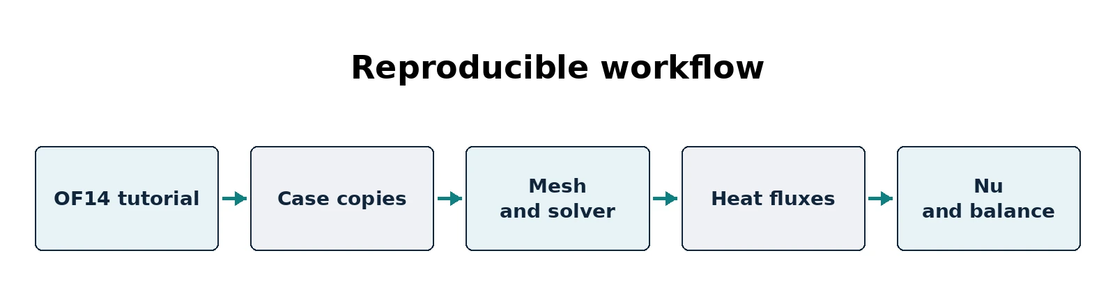
7. Prepare two experiments without touching the tutorial
The supplied scripts/prepare_cases.py reads the installed official tutorial and creates two new, independent directories. It checks that the expected hot and cold wall temperatures match the verified OpenFOAM 14 source. If the destination exists, it refuses to overwrite it.
From Windows PowerShell, open an SSH session:
ssh USER@SERVER_IPTransfer the scripts/ folder using FileZilla, then run the following within an OpenFOAM 14 shell on Linux:
foamVersion
python3 scripts/prepare_cases.py \
  --source "$FOAM_TUTORIALS/fluid/buoyantCavity" \
  --dest "$HOME/OpenFOAM/guide10_thermal_study"
find "$HOME/OpenFOAM/guide10_thermal_study" -maxdepth 2 -type d
You will obtain baseline_19p6K and hotter_29p6K. Do not create your working study inside the OpenFOAM installation or the original tutorials directory.
Deep dive · Package script: prepare_cases.py
#!/usr/bin/env python3
# SPDX-License-Identifier: GPL-3.0-or-later
"""Create non-destructive OpenFOAM 14 buoyantCavity thermal study cases."""
import argparse
import os
from pathlib import Path
import re
import shutil
import sys


def update_hot_temperature(text: str, new_temp: float) -> str:
    # This parser is intentionally constrained to the verified OF14 tutorial input.
    pattern = r'(\bhot\s*\{[^{}]*?\bvalue\s+uniform\s+)([0-9.+eE-]+)(\s*;)'
    matches = list(re.finditer(pattern, text, re.DOTALL))
    if len(matches) != 1 or float(matches[0].group(2)) != 307.75:
        raise ValueError('Unexpected hot patch: tutorial version differs from verified OF14 source')
    return re.sub(pattern, lambda m: m.group(1) + format(new_temp, '.2f') + m.group(3), text, count=1, flags=re.DOTALL)


def main():
    parser = argparse.ArgumentParser(description=__doc__)
    parser.add_argument('--source', type=Path, default=Path(os.environ.get('FOAM_TUTORIALS', '')) / 'fluid/buoyantCavity', help='Official OF14 buoyantCavity source directory')
    parser.add_argument('--dest', type=Path, required=True, help='New, nonexisting study directory')
    args = parser.parse_args()
    source = args.source.expanduser().resolve()
    dest = args.dest.expanduser().resolve()
    if not (source/'0/T').is_file() or not (source/'system/controlDict').is_file():
        parser.error('Official tutorial source not found: load OpenFOAM 14 shell first')
    if dest.exists():
        parser.error(f'Destination already exists; refusing to overwrite: {dest}')
    temp_data = (source/'0/T').read_text(encoding='utf-8')
    if 'uniform 288.15' not in temp_data:
        parser.error('Unexpected cold-wall temperature in source tutorial')
    # Validate before creating anything.
    baseline_text = update_hot_temperature(temp_data, 307.75)
    hot_text = update_hot_temperature(temp_data, 317.75)
    dest.mkdir(parents=True)
    for name, content in (('baseline_19p6K', baseline_text), ('hotter_29p6K', hot_text)):
        target = dest/name
        shutil.copytree(source, target, ignore=shutil.ignore_patterns('processor*', 'postProcessing', 'log.*'))
        (target/'0/T').write_text(content, encoding='utf-8')
    print(f'Created two independent cases in {dest}')
    print('Baseline: Th=307.75 K, Tc=288.15 K, dT=19.60 K')
    print('Hotter:   Th=317.75 K, Tc=288.15 K, dT=29.60 K')


if __name__ == '__main__':
    try:
        main()
    except (ValueError, OSError) as exc:
sys.exit(f'ERROR: {exc}')- The regular expression looks, inside the
hotblock, for the linevalue uniform …;; if there is not exactly one occurrence or the value is not 307.75, it stops: this protects against tutorials from other versions. - Both versions of
0/Tare built and validated before any folder is created. shutil.ignore_patterns('processor*', 'postProcessing', 'log.*')avoids copying results of previous runs in the source folder.- If the destination exists,
parser.errorexits with code 2 without touching anything.
Practical tip · A third copy for experiments
The monitoring function objects (section 8), the Prt file (section 4) or a finer mesh (section 13) belong in additional copies, not in the two reference ones. The script accepts any new destination:
python3 scripts/prepare_cases.py \
  --source "$FOAM_TUTORIALS/fluid/buoyantCavity" \
  --dest "$HOME/OpenFOAM/guide10_thermal_study_monitor"
# then edit only baseline_19p6K inside the new folder, before running it
Record in the study log which copy contains which change and check it with diff -ru against the tutorial.
8. Execute the cases and read the logs
For each newly created case:
bash scripts/run_case.sh \
  "$HOME/OpenFOAM/guide10_thermal_study/baseline_19p6K"
Check this baseline before executing the hotter_29p6K variant. The script runs blockMesh, checkMesh, and foamRun, storing logs under logs/; it also attempts optional wallHeatFlux post-processing. It never deletes existing data and refuses to launch on already meshed or logged cases. Prepare a fresh copy or manually inspect the failed run before retrying.
For longer jobs, use tmux (Guide 1). To inspect a running solver from another terminal:
tail -n 35 "$HOME/OpenFOAM/guide10_thermal_study/baseline_19p6K/logs/foamRun.log"Review residuals, thermal-field behaviour, property-model errors and solver termination. A numerically stable log is not sufficient to establish a consistent thermal energy balance.
Deep dive · Package script: run_case.sh
#!/usr/bin/env bash
# SPDX-License-Identifier: GPL-3.0-or-later
# Run an untouched study case exactly once; preserve all existing outputs.
set -euo pipefail
if [[ $# -ne 1 ]]; then
  echo 'Usage: run_case.sh /absolute/path/to/new/case' >&2
  exit 2
fi
CASE_DIR=$(realpath -- "$1")
[[ -f "$CASE_DIR/system/controlDict" ]] || { echo 'Invalid case' >&2; exit 2; }
command -v foamRun >/dev/null || { echo 'Load the OpenFOAM 14 environment first' >&2; exit 2; }
if [[ -e "$CASE_DIR/logs" || -e "$CASE_DIR/constant/polyMesh" ]]; then
  echo 'Case already has logs or a mesh. Refusing to rerun or overwrite it.' >&2
  exit 3
fi
mkdir "$CASE_DIR/logs"
cd "$CASE_DIR"
blockMesh > logs/blockMesh.log 2>&1
checkMesh > logs/checkMesh.log 2>&1
foamRun > logs/foamRun.log 2>&1
# Optional post-process. Its failure does not change the solver success state.
if command -v foamPostProcess >/dev/null; then
  if ! foamPostProcess -latestTime -func wallHeatFlux > logs/wallHeatFlux.log 2>&1; then
    echo 'Warning: wallHeatFlux post-processing failed; review logs/wallHeatFlux.log' >&2
  fi
fi
echo "Solver completed. Logs are in $CASE_DIR/logs"
set -euo pipefail: the script stops at the first failed command, on undefined variables and on pipeline errors; so ifcheckMeshfails,foamRundoes not start.- The check on
logsandconstant/polyMeshprevents re-running a case already launched (exit code 3). - The
wallHeatFluxpost-processing is inside anif !: a failure only produces a warning and does not cancel the solver success. - The script does not run
sample: for the comparison with experimental data see section 10.
Practical tip · Converged or stopped? Read it in the log
cd "$HOME/OpenFOAM/guide10_thermal_study/baseline_19p6K"
grep -c "^Time = " logs/foamRun.log            # iterations performed
grep -n -i "converged" logs/foamRun.log | tail -3
grep "Solving for h" logs/foamRun.log | tail -3  # h residuals
tail -n 5 logs/foamRun.log                      # must end with End
If the number of iterations is 1000 and no convergence message appears, the run was stopped by endTime. To extract residual histories without disturbing the case logs/ folder, run foamLog from a separate folder, because it creates its own logs subfolder in the current directory:
mkdir "$HOME/OpenFOAM/guide10_thermal_study/foamLog_baseline"
cd "$HOME/OpenFOAM/guide10_thermal_study/foamLog_baseline"
foamLog ../baseline_19p6K/logs/foamRun.log
ls logs/   # h_0, p_rgh_0, Ux_0 ... one column per iteration
Deep dive · Following Q during the run with a system/functions file
OpenFOAM 14 automatically reads the file system/functions, if present, in addition to any functions entry in controlDict. In a new copy, before run_case.sh, save this file as system/functions:
/*--------------------------------*- C++ -*----------------------------------*\
  Guide 10 - monitoring functions for a NEW copy of buoyantCavity.
  Save as <case>/system/functions before running the solver.
\*---------------------------------------------------------------------------*/
FoamFile
{
    format      ascii;
    class       dictionary;
    location    "system";
    object      functions;
}

// Integrated wall heat flow Q [W] on the hot and cold walls every 10 iterations.
// Positive values: heat entering the fluid. No field is written (writeFields false).
wallHeatFluxMonitor
{
    type            wallHeatFlux;
    libs            ("libfieldFunctionObjects.so");
    patches         (hot cold);
    executeControl  timeStep;
    executeInterval 10;
    writeControl    timeStep;
    writeInterval   10;
    writeFields     false;
    log             yes;
}

// Initial residuals of the solved fields, one line per iteration.
#includeFunc residuals(p_rgh, U, h, k, omega)

// Maximum velocity magnitude: a cheap indicator of the circulation strength.
#includeFunc cellMaxMag(name=UmaxMag, U)

// ************************************************************************* //
The syntax is that of the official version 14 tutorials (fluid/concentricCylinders, multiRegion/CHT/wallBoiling); writeFields false avoids writing the wallHeatFlux field at each execution. The result is a file postProcessing/wallHeatFluxMonitor/0/wallHeatFlux.dat with one line per patch every 10 iterations, readable with whf_extract.py (section 9): the evolution of Qhot and Qcold is the physically meaningful convergence criterion. At start-up the log must show the creation of the three function objects; if one is missing, check the file header.
9. Wall heat flux using wallHeatFlux
OpenFOAM 14 provides the wallHeatFlux function object for evaluating heat fluxes on wall patches. A non-invasive post-processing attempt is:
foamPostProcess -case \
  "$HOME/OpenFOAM/guide10_thermal_study/baseline_19p6K" \
  -latestTime -func wallHeatFlux
run_case.sh also attempts this command but reports post-processing failures separately from solver completion. If an explicit function-object dictionary is needed for your installation, consult foamInfo wallHeatFlux and the Foundation 14 class reference.
A heat-flux density [W/m²] becomes thermal power [W] only after surface integration: Q = ∫_A q'' dA. Check signs, wall normals, data association, and units before integrating. The arithmetic average of patch values is not the same as the integrated wall power.
Deep dive · What wallHeatFlux computes, read in the source
From the OpenFOAM 14 file src/functionObjects/field/wallHeatFlux/wallHeatFlux.C:
- the field is minus the transport-model heat flux on the boundary face,
wallHeatFlux = −q, where q is positive along the outward normal of the domain. Hence wallHeatFlux > 0 means heat entering the fluid through the wall; - if a radiative field
qrexists it is subtracted too, so the result includes radiation when modelled; - for each patch min, max, the integrated power
Q = Σ |S<sub>f</sub>| q[W] and the area averageq = Q/Σ|S<sub>f</sub>|[W/m²] are written, both in the log and in the filepostProcessing/<name>/<time>/wallHeatFlux.dat; - without a
patchesentry all patches of typewallare processed.
So the integration of section 9 is already done by OpenFOAM, on the actual mesh and with the exact face areas: Qhot is the Q value of the hot patch, Qcold is the Q value of the cold patch with its sign changed. The adiabatic patches, with zeroGradient, must give Q = 0. ParaView remains useful as an independent check and for the local distribution.
Practical tip · If wallHeatFlux.log reports an error: add -solver fluid
In the foamPostProcess source (version 14) the physical models are constructed only when the solver is given with -solver; otherwise the utility only reads fields. wallHeatFlux needs the thermal transport model and, if it cannot find it, stops with “Unable to find thermophysicalTransportModel”. This is exactly the situation in which run_case.sh prints its warning without compromising the run. Check and, if needed, repeat with the explicit solver and a new log name:
cd "$HOME/OpenFOAM/guide10_thermal_study/baseline_19p6K"
grep -i "error\|unable" logs/wallHeatFlux.log
foamPostProcess -solver fluid -latestTime -func wallHeatFlux > logs/wallHeatFlux_solver.log 2>&1
grep "for patch" logs/wallHeatFlux_solver.log
In the output look for the lines “min, max, Q [W], q [W/m^2] for patch hot = …” and “… for patch cold = …”: the third number is the integrated power. The same applies to yPlus and to every function object that needs the turbulence or thermal transport model; sample, instead, only reads T and U and works without -solver, as in the official Allrun.
Deep dive · Additional script: whf_extract.py
Reads one or more wallHeatFlux.dat files, converts signs to the guide convention, shows the signed sum over all patches (it must tend to zero at convergence), the drift of Qhot over the last records and, on request, writes the measurement row for thermal_balance.py:
cd "$HOME/OpenFOAM/guide10_thermal_study/baseline_19p6K"
find postProcessing -name wallHeatFlux.dat
python3 whf_extract.py postProcessing/wallHeatFlux/*/wallHeatFlux.dat \
  --case baseline_19p6K --Th 307.75 --Tc 288.15 \
  --output ../baseline_measurements.csv
python3 scripts/thermal_balance.py ../baseline_measurements.csv ../baseline_results.csv
#!/usr/bin/env python3
# SPDX-License-Identifier: GPL-3.0-or-later
"""Read OpenFOAM 14 wallHeatFlux.dat files and prepare a thermal_balance.py row.
The wallHeatFlux function object writes, for every processed time and wall
patch: Time, patch, min [W/m2], max [W/m2], Q [W], q [W/m2]. In OpenFOAM 14 the
field is minus the boundary heat flux along the outward normal, so a positive Q
means heat entering the fluid through that patch. This tool converts the raw
signed values to the positive Q_hot / Q_cold convention of Guide 10, reports the
sum over all wall patches and, when several times are present, the drift of Q
over the last records. It never overwrites an existing output file.
"""
import argparse
import csv
from collections import OrderedDict
from pathlib import Path
import sys
def read_dat(paths):
data = OrderedDict() # time -> {patch: Q}
for path in paths:
with open(path, encoding='utf-8') as f:
for number, line in enumerate(f, 1):
s = line.strip()
if not s or s.startswith('#'):
continue
parts = s.split()
if len(parts) < 6:
raise ValueError(f'{path}:{number}: expected 6 columns, found {len(parts)}')
t, patch, q_total = float(parts[0]), parts[1], float(parts[4])
data.setdefault(t, {})[patch] = q_total
if not data:
raise ValueError('No data rows found')
return OrderedDict(sorted(data.items()))
def main():
p = argparse.ArgumentParser(description=__doc__)
p.add_argument('dat', nargs='+', type=Path, help='wallHeatFlux.dat file(s)')
p.add_argument('--case', required=True, help='case label for the output row')
p.add_argument('--hot', default='hot', help='hot patch name')
p.add_argument('--cold', default='cold', help='cold patch name')
p.add_argument('--Th', type=float, required=True, help='hot wall temperature [K]')
p.add_argument('--Tc', type=float, required=True, help='cold wall temperature [K]')
p.add_argument('--area-hot', type=float, default=1.1336, help='hot wall area [m2]')
p.add_argument('--area-cold', type=float, default=1.1336, help='cold wall area [m2]')
p.add_argument('--L', type=float, default=0.076, help='characteristic length [m]')
p.add_argument('--k', type=float, default=0.026086, help='fluid conductivity [W/(m K)]')
p.add_argument('--last', type=int, default=10, help='records used for the drift check')
p.add_argument('--output', type=Path, help='NEW csv for thermal_balance.py')
a = p.parse_args()
data = read_dat(a.dat)
t_last, row = next(reversed(data.items()))
for name in (a.hot, a.cold):
if name not in row:
p.error(f'patch {name} not found at time {t_last}; available: {", ".join(row)}')
q_hot, q_cold = row[a.hot], -row[a.cold]
print(f'Last time: {t_last:g} ({len(data)} time records)')
for name, value in row.items():
print(f' raw Q[{name}] = {value:+.6g} W')
print(f'Q_hot = {q_hot:.6g} W (heat entering the fluid)')
print(f'Q_cold = {q_cold:.6g} W (heat leaving the fluid)')
print(f'Sum of signed Q over all wall patches = {sum(row.values()):+.6g} W')
if q_hot <= 0 or q_cold <= 0:
print('WARNING: unexpected sign; check patch names and the sign convention before continuing')
if len(data) > 1:
tail = list(data.items())[-max(2, a.last):]
series = [r[a.hot] for _, r in tail if a.hot in r]
ref = max(abs(v) for v in series)
drift = (max(series) - min(series)) / ref * 100 if ref else float('nan')
print(f'Drift of Q[{a.hot}] over the last {len(series)} records: {drift:.3g} %')
if a.output:
if a.output.exists():
p.error('Output already exists; refusing to overwrite it')
with a.output.open('x', newline='', encoding='utf-8') as f:
w = csv.writer(f)
w.writerow(['case', 'Th_K', 'Tc_K', 'Ahot_m2', 'Acold_m2', 'Qhot_W', 'Qcold_W', 'L_m', 'k_W_mK'])
w.writerow([a.case, a.Th, a.Tc, a.area_hot, a.area_cold, f'{q_hot:.6g}', f'{q_cold:.6g}', a.L, a.k])
print('Measurement row written to', a.output)
if __name__ == '__main__':
try:
main()
except (OSError, ValueError) as exc:
sys.exit(f'ERROR: {exc}')Tested on a file built with the format written by the source (columns Time, patch, min, max, Q, q): with Q(hot) = 36.5 W and Q(cold) = −35.8 W it returns Qhot = 36.5 W, Qcold = 35.8 W, sum +0.7 W, and the row it produces gives Nuhot = 4.786 in thermal_balance.py with k = 0.026086. It refuses an existing output file and a non-existent patch.
Deep dive · Wall heat flux depends on the wall model
On the wall face the flux is computed as κeff ∂T/∂n with κeff = κ + cp αt,w, where αt,w comes from alphatWallFunction with Prt = 0.85, and the normal gradient is evaluated between the first cell centre and the wall. If the first-cell y⁺ is of order 1–2, νt at the wall is almost zero and the flux is essentially molecular; if the mesh is coarser, the wall function replaces the missing part of the profile with a universal law, which for natural convection is less reliable than for forced boundary layers. Nu must always be reported together with the first-cell y⁺ and the mesh used.
Practical tip · Computing y⁺ on the thermal walls
cd "$HOME/OpenFOAM/guide10_thermal_study/baseline_19p6K"
foamPostProcess -solver fluid -latestTime -func yPlus > logs/yPlus.log 2>&1
grep -A4 "patch hot\|patch cold" logs/yPlus.log
The yPlus function object prints minimum, maximum and average for each wall patch and writes the yPlus field, which can be viewed in ParaView along the height. The log name is new, so nothing is overwritten; if it already exists, choose another.
10. Quantitative measurements from Windows ParaView
Open the case using ParaView connected to the Linux pvserver (Guides 1 and 3). Load T, U, and wallHeatFlux if this field was generated.
- Make a Slice through the middle of the cavity depth and colour by
Tto inspect thermal gradients and stratification. - Use Glyph or Stream Tracer for
Uto inspect buoyancy-driven circulation; document seeds, scale, and selected time. - Select the
hotandcoldpatches using Extract Surface or the corresponding patch blocks; apply Integrate Variables to obtain integrated thermal power. - Use Save Data to export final measurements as CSV, including the reported time and a clearly stated heat-flux sign convention.
Do not automatically substitute a cell-centred Gradient filter for a numerical wall-flux evaluation: boundary extrapolation and discretized wall conditions may produce differences.
Deep dive · Integrate Variables: the settings that change the result
- Select only the patch in the OpenFOAM reader (in the “Mesh Regions” list patches appear with the prefix
patch/), or isolate it with Extract Block: integrating the whole volume produces a meaningless number. - Integrate the cell array
wallHeatFlux: by default the reader also creates interpolated point values, which on the boundary do not coincide with face values. - Leave “Divide Cell Data By Volume” off: with the option on the filter returns an average, not an integral.
- The filter also reports
Area: for the hot wall it must be 1.1336 m². A different value reveals a wrong selection. - The integrated value must match, up to rounding, the Q printed by
wallHeatFluxfor the same patch and time.
Deep dive · Additional script: compare_expt.py
After generating the profiles with the tutorial sample function object, the script compares T and vertical velocity with the Betts and Bokhari data by interpolating the computation at the experimental abscissae and reporting mean, RMS and maximum deviation for each height:
cd "$HOME/OpenFOAM/guide10_thermal_study/baseline_19p6K"
foamPostProcess -latestTime -func sample > logs/sample.log 2>&1
ls postProcessing/sample/*/
python3 compare_expt.py . --output ../baseline_vs_expt.csv
#!/usr/bin/env python3
# SPDX-License-Identifier: GPL-3.0-or-later
"""Compare buoyantCavity sample profiles with the Betts & Bokhari data.
Reads postProcessing/sample/<latest time>/y0.<i>.xy written by
'foamPostProcess -latestTime -func sample' (columns: x T Ux Uy Uz, as assumed by
the tutorial's validation/createGraphs script) and the experimental files
validation/exptData/mt_z0_<i>0_lo.dat (x [mm], T [degC]) and
mv_z0_<i>0_lo.dat (x [mm], Uy [m/s]). The simulated profile is linearly
interpolated at each experimental abscissa. Prints mean, RMS and maximum
deviations per height and optionally writes them to a NEW CSV file.
"""
import argparse
import csv
import math
from pathlib import Path
import sys
def read_columns(path):
rows = []
with open(path, encoding='utf-8') as f:
for line in f:
s = line.strip()
if not s or s.startswith('#'):
continue
rows.append([float(v) for v in s.split()])
if not rows:
raise ValueError(f'No numeric data in {path}')
return rows
def interp(xs, ys, x):
if x < xs[0] or x > xs[-1]:
return None
for i in range(1, len(xs)):
if x <= xs[i]:
x0, x1, y0, y1 = xs[i - 1], xs[i], ys[i - 1], ys[i]
return y0 if x1 == x0 else y0 + (y1 - y0) * (x - x0) / (x1 - x0)
return ys[-1]
def stats(diffs):
n = len(diffs)
mean = sum(diffs) / n
rms = math.sqrt(sum(d * d for d in diffs) / n)
worst = max(diffs, key=abs)
return n, mean, rms, worst
def latest_time_dir(root):
dirs = []
for d in root.iterdir():
try:
dirs.append((float(d.name), d))
except ValueError:
continue
if not dirs:
raise ValueError(f'No time directories in {root}')
return max(dirs)[1]
def main():
p = argparse.ArgumentParser(description=__doc__)
p.add_argument('case', type=Path, help='case directory containing postProcessing/sample')
p.add_argument('--expt', type=Path, help='experimental data directory (default: <case>/validation/exptData)')
p.add_argument('--output', type=Path, help='NEW csv summary file')
a = p.parse_args()
expt = a.expt or a.case / 'validation' / 'exptData'
sdir = latest_time_dir(a.case / 'postProcessing' / 'sample')
print('Simulation profiles from', sdir)
if a.output and a.output.exists():
p.error('Output already exists; refusing to overwrite it')
results = []
for i in range(1, 10):
sim_file = sdir / f'y0.{i}.xy'
if not sim_file.is_file():
continue
sim = sorted(read_columns(sim_file))
xs = [r[0] for r in sim]
for kind, col, fname, conv, unit in (('T', 1, f'mt_z0_{i}0_lo.dat', 273.15, 'K'),
('Uy', 3, f'mv_z0_{i}0_lo.dat', 0.0, 'm/s')):
efile = expt / fname
if not efile.is_file():
continue
ys = [r[col] for r in sim]
diffs = []
for row in read_columns(efile):
value = interp(xs, ys, row[0] / 1000.0)
if value is not None:
diffs.append(value - (row[1] + conv))
if not diffs:
continue
n, mean, rms, worst = stats(diffs)
results.append(dict(y_over_H=f'0.{i}', quantity=kind, unit=unit, points=n,
mean_dev=f'{mean:.4g}', rms_dev=f'{rms:.4g}', max_abs_dev=f'{worst:.4g}'))
print(f'y/H=0.{i} {kind:2s}: n={n:2d} mean={mean:+.4g} {unit} rms={rms:.4g} {unit} worst={worst:+.4g} {unit}')
if not results:
p.error('No matching simulation/experiment pairs found')
if a.output:
with a.output.open('x', newline='', encoding='utf-8') as f:
w = csv.DictWriter(f, fieldnames=list(results[0]))
w.writeheader()
w.writerows(results)
print('Summary written to', a.output)
print('Deviation = simulation - experiment. The data come from the tutorial; cite the original publication.')
if __name__ == '__main__':
try:
main()
except (OSError, ValueError) as exc:
sys.exit(f'ERROR: {exc}')The script assumes the “x T Ux Uy Uz” column format of the y0.N.xy files, the same used by the tutorial validation/createGraphs (column 4 for Uy): if ls shows different names or columns, adapt the indices before using it. It was tested on hand-built profiles and on the tutorial’s real experimental files. Deviations of a few tenths of a kelvin in the core and 1–2 K near the walls are typical of RANS computations of this case; deviations of many kelvin indicate a problem.
Practical tip · Comparable profiles in ParaView
- To compare visually with experimental data use Plot Over Line from (0, y, 0) to (0.076, y, 0) with y = 1.09 m (y/H = 0.5): these are the same coordinates as the
y0.5line insystem/sample. - Set the same colour scale (for example 288–318 K) for both cases and save it as a preset: comparisons between images with different scales have no value.
- For stratification, a vertical Plot Over Line at the centre (x = 0.038 m, z = 0) shows T versus height: in tall cavities the core is approximately linearly stratified.
- Save the state with File → Save State (
.pvsm) next to the exported CSV files.
11. From thermal power to the Nusselt number
Define Q_hot > 0 as power entering the fluid through the hot wall and Q_cold > 0 as power leaving the fluid through the cold wall. Each principal wall area in the official geometry is A = 2.18 × 0.52 = 1.1336 m².
Choose the declared characteristic length as the wall separation, L = 0.076 m:
Nuhot = ( Qhot / Ahot ) L / [ k ( Thot − Tcold ) ]
A relative steady-state energy imbalance based on two positive powers is:
εE = 100 · | Qhot − Qcold | / max( Qhot, Qcold ) %
Important: tall-cavity publications may use alternative characteristic lengths, including the cavity height. A Nusselt number computed using the gap width is not directly comparable with a height-based definition. Raw wall-flux signs must first be converted, with documented surface normals, into the positive Q_hot and Q_cold conventions defined here.
Deep dive · Nusselt: definitions, references and a check on the experimental data
| Definition | Formula | Comment |
|---|---|---|
| NuW | q̄ W / (κ ΔT) | the guide’s; NuW = 1 is pure conduction |
| NuH | q̄ H / (κ ΔT) = NuW · H/W | 28.7 times larger for the same flux |
| local Nu Nu(y) | q(y) W / (κ ΔT) | from the wallHeatFlux field along the height |
An independent check comes from the tutorial data: at mid-height near the cold wall the measured temperature goes from 15.0 °C (wall) to 15.62 °C at 0.33 mm, then 15.94 °C at 0.58 mm and 16.45 °C at 0.84 mm. The near-wall gradient is therefore between 1.3 and 2 K/mm, i.e. a local Nu between about 5 and 7.5. This is consistent with the correlation NuW ≈ 5.65 and with the synthetic value 4.79 of the figure: the order of magnitude is right, precise numbers must come from the computation. The mean value measured by Betts and Bokhari for this ΔT, reported by the ERCOFTAC sheet, is Nu = 5.85: it is the experimental reference against which to compare Nuhot and Nucold, after checking in the source that the definition (length W, conductivity, ΔT) matches the definition used here.
Deep dive · Uncertainty propagation for Nu
For Nu = Q L / (A κ ΔT), with independent quantities, the relative uncertainty is:
(dNu/Nu)^2 = (dQ/Q)^2 + (dL/L)^2 + (dA/A)^2 + (dk/k)^2 + (d(DeltaT)/DeltaT)^2In a simulation L, A and ΔT are exact by construction; κ is an input (model uncertainty, not numerical); the dominant term is dQ/Q, to be estimated as a combination of: difference between Qhot and Qcold, iterative drift over the last iterations and difference between meshes (section 13). For the central value use the mean (Qhot + Qcold)/2 and report half the difference as one component of the uncertainty.
Practical tip · Local Nu along the height
In ParaView, on the hot patch, use a Calculator on cell data with the expression wallHeatFlux*0.076/(0.026086*19.6) named Nu_local; then Plot Data or Plot Over Line along y at z = 0. The expected curve is high at the bottom, where the hot boundary layer starts, and decreases upwards; for the cold wall the trend is mirrored (and values are negative because of the sign convention). The area average of Nu_local must equal Nuhot computed from Q.
12. Exercise: measurements, CSV and thermal balance
The bundle contains examples/measurement_TEMPLATE.csv (empty rows) and example_MEASUREMENTS_SYNTHETIC.csv (invented numbers for software tests only). After exporting real ParaView measurements, fill in Th_K, Tc_K, Ahot_m2, Acold_m2, Qhot_W, Qcold_W, L_m, and k_W_mK. Then run on Windows or Linux:
python scripts/thermal_balance.py examples/measurement_TEMPLATE.csv results.csvNote: the template contains just a header: add at least one measurement record before running this command. To test the tool immediately without CFD data:
python scripts/thermal_balance.py examples/example_MEASUREMENTS_SYNTHETIC.csv examples/test_results.csvThe script computes Nu_hot, Nu_cold, and the energy-balance error. It does not invent CFD measurements and refuses to overwrite an existing output file. Never present the synthetic records as actual computational or experimental findings.
Deep dive · Package script: thermal_balance.py
#!/usr/bin/env python3
# SPDX-License-Identifier: GPL-3.0-or-later
"""Evaluate signed wall-power magnitudes, balance error, and cavity Nusselt number."""
import argparse
import csv
from pathlib import Path
import sys

REQUIRED = ('case', 'Th_K', 'Tc_K', 'Ahot_m2', 'Acold_m2', 'Qhot_W', 'Qcold_W', 'L_m', 'k_W_mK')


def evaluate(row):
    label = row['case'].strip()
    if not label:
        raise ValueError('Empty case name')
    values = {}
    for col in REQUIRED[1:]:
        values[col] = float(row[col])
    th, tc = values['Th_K'], values['Tc_K']
    ah, ac = values['Ahot_m2'], values['Acold_m2']
    qh, qc = values['Qhot_W'], values['Qcold_W']
    gap, k = values['L_m'], values['k_W_mK']
    if not th > tc or min(ah, ac, qh, qc, gap, k) <= 0:
        raise ValueError('Expected Th > Tc and strictly positive areas, powers, gap, conductivity')
    denom = k * (th - tc)
    return dict(case=label, deltaT_K=f'{th-tc:.6g}', Nu_hot=f'{qh*gap/ah/denom:.6g}',
                Nu_cold=f'{qc*gap/ac/denom:.6g}',
                relative_imbalance_percent=f'{100*abs(qh-qc)/max(qh,qc):.6g}',
                Qhot_W=f'{qh:.6g}', Qcold_W=f'{qc:.6g}')


def main():
    parser = argparse.ArgumentParser(description=__doc__)
    parser.add_argument('input_csv', type=Path)
    parser.add_argument('output_csv', type=Path)
    args = parser.parse_args()
    if args.output_csv.exists():
        parser.error('Output already exists; refusing to overwrite it')
    with args.input_csv.open(newline='', encoding='utf-8-sig') as f:
        reader = csv.DictReader(f)
        if not set(REQUIRED).issubset(set(reader.fieldnames or [])):
            parser.error('CSV missing required columns: ' + ', '.join(REQUIRED))
        rows = [evaluate(row) for row in reader]
    if not rows:
        parser.error('Empty data table')
    with args.output_csv.open('x', newline='', encoding='utf-8') as f:
        writer = csv.DictWriter(f, fieldnames=list(rows[0]))
        writer.writeheader()
        writer.writerows(rows)
    for row in rows:
        print(f"{row['case']}: Nu_hot={row['Nu_hot']}, Nu_cold={row['Nu_cold']}, balance error={row['relative_imbalance_percent']}%")
    print('Results saved:', args.output_csv)


if __name__ == '__main__':
    try:
        main()
    except (OSError, ValueError, KeyError) as exc:
sys.exit(f'ERROR: {exc}')- Required columns:
case, Th_K, Tc_K, Ahot_m2, Acold_m2, Qhot_W, Qcold_W, L_m, k_W_mK; the Excel BOM is handled byutf-8-sig. - It rejects Th ≤ Tc and any non-positive area, power, gap or conductivity: this is why Qcold must be entered already positive.
- The output file is opened in
'x'mode: if it exists, the operation fails instead of overwriting. - Run on the package synthetic file it produces a file identical to
examples/derived_SYNTHETIC.csv(Nuhot 4.78722 and 5.29766, imbalances 1.91781 % and 0.983607 %); on the empty template it ends with “Empty data table”, as stated in the guide.
Deep dive · Package example files
examples/measurement_TEMPLATE.csv
case,Th_K,Tc_K,Ahot_m2,Acold_m2,Qhot_W,Qcold_W,L_m,k_W_mKexamples/example_MEASUREMENTS_SYNTHETIC.csv (invented data)
case,Th_K,Tc_K,Ahot_m2,Acold_m2,Qhot_W,Qcold_W,L_m,k_W_mK
baseline_SYNTHETIC,307.75,288.15,1.1336,1.1336,36.5,35.8,0.076,0.02608
hotter_SYNTHETIC,317.75,288.15,1.1336,1.1336,61.0,60.4,0.076,0.02608
examples/derived_SYNTHETIC.csv (expected calculator output)
case,deltaT_K,Nu_hot,Nu_cold,relative_imbalance_percent,Qhot_W,Qcold_W
baseline_SYNTHETIC,19.6,4.78722,4.69541,1.91781,36.5,35.8
hotter_SYNTHETIC,29.6,5.29766,5.24555,0.983607,61,60.4
Practical tip · Check the calculator before using it
python scripts/thermal_balance.py examples/example_MEASUREMENTS_SYNTHETIC.csv examples/test_results.csv
fc examples\test_results.csv examples\derived_SYNTHETIC.csv        # Windows
diff examples/test_results.csv examples/derived_SYNTHETIC.csv      # Linux
If the comparison reports no differences, the calculator and the Python interpreter work as expected. Then use a separate folder for real results (for example results/), so synthetic files never mix with measurements.
13. Critical assessment: convergence and uncertainty
Residual convergence alone is not a valid stopping criterion. At a minimum, record the trends in Q_hot and Q_cold, the power imbalance, sensitivity to mesh and thermophysical properties, stability of the convection pattern, Nusselt definition, and near-wall resolution.
Optional refresher — energy balance. For a steady closed cavity with no internal heat source or radiation, total heat entering and leaving should agree within numerical uncertainty. A persistent imbalance can indicate incomplete convergence, flawed flux integration, or errors in units or sign conventions.
The original case uses a three-dimensional mesh and a RANS turbulence model. Do not assume its model choices also apply to laminar natural convection. Increasing the wall-temperature difference may change the flow regime and therefore the requirements for mesh resolution and convergence.
Deep dive · A mesh study targeted at the thermal boundary layer
In a new copy you can refine only near the thermal walls with multi-section grading in the blockMeshDict. Example, where each half of the width has half the cells and a ratio of 4 between the central and the wall cell:
blocks
(
    hex (0 1 2 3 4 5 6 7) (50 150 15)
    simpleGrading
    (
        ((0.5 0.5 4) (0.5 0.5 0.25))   // x: refined at both walls
        1
        1
    )
);
Each triple is (fraction of length, fraction of cells, ratio between last and first cell of the section). Before each run check checkMesh and the first-cell size. A series of three meshes with constant refinement (for example 35, 50 and 70 cells in x, same grading) allows the Richardson method and the GCI of Guide 4 to be applied to Qhot. Keep the number of cells in y and z constant in the first series: changing everything at once confuses the effects.
Deep dive · When the steady computation does not converge
At RaH ≈ 2·10¹⁰ the flow in the tall cavity can show instabilities and low-frequency fluctuations. A steady RANS computation may then oscillate indefinitely between nearby states: residuals stalled on a plateau and Qhot oscillating by a few percent. In this case do not tighten the relaxation factors to “force” convergence; report the oscillation amplitude as iterative uncertainty or, in a new copy, switch to a transient computation (ddtSchemes Euler or backward, time step controlled by the Courant number as in Guide 8) and average quantities over a statistically steady interval.
Practical tip · Sensitivity matrix to document
| Factor | Suggested change | Observed quantity |
|---|---|---|
| mesh in x | 35 → 50 → 70 cells | Qhot, y⁺, Nu |
| bulk Prt | 1 (default) → 0.85 | Qhot |
| turbulence model | kOmegaSST → kEpsilon (with consistent wall functions) | profiles and Q |
| convergence | thresholds 1e-4 → 1e-5 | Q drift |
| ΔT | 19.6 → 29.6 K | Nu (expected growth roughly as Ra0.3) |
Change one factor at a time, each in its own copy, and report the results in a single table. With the 0.293 exponent of the correlation, going from ΔT = 19.6 to 29.6 K one expects NuW about 13 % higher: a very different increase needs an explanation.
14. Suggested extensions
- Forced convection in a duct: prescribe inlet
UandT, heat a wall, and compare the measured power with the enthalpy increasemass_flow * Cp * (Tout-Tin). Use suitable liquid properties rather than copying ideal-gas thermodynamics without justification. - Conjugate heat transfer: separate fluid and solid regions and use
coupledTemperature, checking that interfacial heat flux is conserved. - External heat transfer: replace a wall condition with
externalTemperaturein a new copy and study sensitivity toh. - Reproducibility: archive
.pvsm, logs, measurement CSVs and exact case dictionaries with software versions and physical assumptions.
Deep dive · Forced convection: analytical references for verification
For the heated-duct extension there are reference solutions that allow a real code verification, not just plausibility:
- fully developed laminar flow in a circular pipe: NuD = 3.66 at constant wall temperature and 4.36 at constant wall flux;
- plane channel between two plates: NuDh = 7.54 (constant temperature) and 8.23 (constant flux) on both walls;
- laminar thermal entry length ≈ 0.05 Re Pr Dh: the domain must be longer to reach the developed value;
- in turbulent flow, correlations such as Gnielinski have 10–20 % uncertainty and only serve as order-of-magnitude comparison.
The balance ṁ cp (Tout − Tin) must use the flow-weighted mean temperature, not the area average: in OpenFOAM 14 it is obtained with a surfaceFieldValue with operation average and weightField phi (procedure described in Guide 11).
Deep dive · Official tutorials useful for the extensions
| Tutorial | What it shows |
|---|---|
fluid/concentricCylinders | integration of wallHeatFlux and of the radiative flux qr on patches with #includeFunc patchIntegrate |
fluid/roomHeating | external wall with externalTemperature and h |
multiRegion/CHT/heatedDuct | the three-region case of Guide 11 |
multiRegion/CHT/vacuumFurnace | mean T in a solid and radiative flux on a patch |
List them all with ls $FOAM_TUTORIALS/fluid $FOAM_TUTORIALS/multiRegion/CHT. Each one’s system/functions file is a good template for your own measurements.
Practical tip · Archiving the study
cd "$HOME/OpenFOAM"
foamVersion > guide10_thermal_study/OPENFOAM_VERSION.txt 2>&1
tar czf guide10_thermal_study_$(date +%Y%m%d).tar.gz guide10_thermal_study
sha256sum guide10_thermal_study_*.tar.gz > guide10_thermal_study_SHA256.txt
The archive is a fingerprinted copy: no file is removed. Keep the measurement CSVs, the thermal_balance.py results, the experimental comparison and the ParaView states together.
15. Scientific checklist
- ☐ All work occurs in a separate user-owned case directory.
- ☐ Wall temperatures are in kelvin and thermophysical properties have been checked.
- ☐
checkMeshand the solver completed without errors, and their logs are stored. - ☐ Wall heat fluxes were integrated with consistent areas and signs.
- ☐
Q_hot,Q_cold, and the relative mismatch have been recorded. - ☐ The Nusselt definition includes
L,k, temperature difference and flux convention. - ☐ Measured values are clearly separated from synthetic demonstration figures.
- ☐ At least convergence and mesh sensitivity have been examined.
Practical tip · Additional checks for research work
- Q of the adiabatic patches equal to zero and signed sum over all patches close to zero.
- “Selecting … thermophysical transport model” line read and Prt declared (wall 0.85, bulk 1 unless set otherwise).
- Number of iterations and reason for stopping (convergence or
endTime) recorded. - First-cell y⁺ on the thermal walls reported.
- Q compared with the correlation estimate (≈ 43 W for the baseline) and deviation explained.
- Profiles compared with the tutorial experimental data, with deviations per height.
- Effect of radiation discussed, at least as an order of magnitude.
- Variant comment corrected or recorded in
hotter_29p6K/0/T.
References and verification limits
- OpenFOAM Foundation 14, official
fluid/buoyantCavitycase: https://github.com/OpenFOAM/OpenFOAM-14/tree/master/tutorials/fluid/buoyantCavity. - OpenFOAM 14 User Guide, thermophysical models: https://doc.cfd.direct/openfoam/user-guide-v14/thermophysical-models.
- OpenFOAM 14 User Guide, thermal boundary conditions: https://doc.cfd.direct/openfoam/user-guide-v14/thermal-boundary-conditions.
- OpenFOAM 14 Source Guide,
wallHeatFlux: https://cpp.openfoam.org/v14/classFoam_1_1functionObjects_1_1wallHeatFlux.html. - OpenFOAM 14 User Guide, post-processing functionality: https://doc.cfd.direct/openfoam/user-guide-v14/post-processing-functionality.
Checks performed for this guide: verification of key official tutorial input files against the Foundation repository, syntax checks of the companion scripts, and calculator execution against synthetic figures. The cases must be executed and assessed on an OpenFOAM 14 server before drawing scientific conclusions.
Original exercise code: GNU GPL version 3 or later. Diagrams are educational; official upstream case files retain their respective licences.
Deep dive · Reference reading, with links
- P. L. Betts, I. H. Bokhari, Experiments on turbulent natural convection in an enclosed tall cavity, International Journal of Heat and Fluid Flow 21(6) (2000) 675–683, doi:10.1016/S0142-727X(00)00033-3: the tutorial experiment (cited in its README);
- Case sheet in the ERCOFTAC database: KBwiki UFR 4-10, natural convection in a tall cavity (geometry, Ra, measured mean Nusselt numbers, downloadable data);
- S. M. ElSherbiny, G. D. Raithby, K. G. T. Hollands, Heat transfer by natural convection across vertical and inclined air layers, Journal of Heat Transfer 104(1) (1982) 96–102, ASME Digital Collection: the correlation used in the estimates;
- I. B. Celik, U. Ghia, P. J. Roache, C. J. Freitas, H. Coleman, P. E. Raad, Procedure for estimation and reporting of uncertainty due to discretization in CFD applications, Journal of Fluids Engineering 130 (2008) 078001, text published by ASME: the GCI used in the mesh study;
- T. L. Bergman, A. S. Lavine, F. P. Incropera, D. P. DeWitt, Fundamentals of Heat and Mass Transfer, 8th ed., Wiley, 2017 (ISBN 978-1-119-35388-1), Wiley: natural convection in enclosures, surface radiation, forced convection in ducts;
- A. Bejan, Convection Heat Transfer, 4th ed., Wiley, 2013 (ISBN 978-0-470-90037-6): scale analysis of natural-convection boundary layers;
- F. R. Menter, Two-equation eddy-viscosity turbulence models for engineering applications, AIAA Journal 32(8) (1994) 1598–1605: the tutorial k-ω SST model (Guide 9).
The tutorial README also gives the ERCOFTAC/Manchester database page (case 79) the experimental data come from.
Deep dive · The OpenFOAM 14 source files cited in the boxes
Every statement about the behaviour of the code can be checked directly in the official Foundation repository:
- tutorials/fluid/buoyantCavity — the complete case, with
validation/exptDataandsystem/sample - applications/modules/fluid/thermophysicalPredictor.C — energy equation of the fluid module
- src/finiteVolume/cfdTools/general/buoyancy/buoyancy.H — definition of p_rgh, gh, pRef and hRef
- src/functionObjects/field/wallHeatFlux/wallHeatFlux.C — flux sign and integrated power Q
- RASThermophysicalTransportModel.C + unityLewisEddyDiffusivity.C — default model and Prt = 1
- externalTemperatureFvPatchScalarField.H — Q, q, h, Ta, emissivity options
- src/thermophysicalModels/specie/thermo/hConst/hConstThermo.H — sensible enthalpy and Tref
- foamPostProcess.C — the -solver option and model construction
- etc/caseDicts/functions — the configurations used by #includeFunc and -func
Related guides: Linux server from Windows, monitoring and convergence, ParaView for quantitative analysis, verification and validation, parameter sweeps, mesh generation and quality checks, boundary conditions and physical models, transient simulations, turbulence and RANS models and the Learning OpenFOAM 14 path.