

OpenFOAM: turbulence, k-ε and k-ω SST RANS models and near-wall treatment
Ninth guide of the Learning OpenFOAM 14 path and the first of the “Turbulence, heat and mass” module of the advanced course, after those on server and transfers, monitoring and convergence, quantitative analysis with ParaView, verification and validation, parameter sweeps, mesh generation, boundary conditions and models and transient simulations. This one tackles turbulence: k-ε and k-ω SST RANS models compared, inlet conditions, wall functions and y⁺, reattachment and pressure losses. The deep-dive and practical-tip boxes open with a click: they contain every package script, the numerical estimates for the case, two additional scripts for y⁺ and reattachment, and verification procedures.
From k-ε and k-ω SST to y+ verification, separated flow and quantitative comparisons
OpenFOAM practical guide series · Linux server, Windows client · English edition
Goal: configure and compare two RANS models on the same geometry, checking inlet conditions, wall functions, mesh requirements and physical quantities. This guide targets OpenFOAM Foundation 14 and ParaView 5.13.2. Windows-side applications are PowerShell, FileZilla, Notepad++ and ParaView. Illustrations are conceptual, not actual CFD results.
1. Why turbulence needs its own guide
Numerical convergence does not establish physical validity. In turbulent flows, velocity fluctuations transport momentum over many spatial and temporal scales. A RANS mesh does not explicitly resolve those fluctuations; a closure model represents their mean effect. Different closures can produce different pressure drops, friction, separation lengths and velocity recovery downstream of an obstacle.
A sound comparison asks more than “which model converges?” It asks which physical quantity is predicted, at what uncertainty, and with what evidence? Boundary conditions, mesh resolution and wall treatment must be controlled before model discrepancies can be meaningfully interpreted.
Optional refresher — Reynolds number. Re = U L / ν compares inertia to viscous effects. Its transition threshold is not universal: it depends on geometry, inlet disturbances and wall roughness. Do not select a turbulence model using an unrelated smooth-pipe transition criterion.
Deep dive · The dimensionless numbers of the case, before any model
With the tutorial data (U = 10 m/s, ν = 1·10⁻⁵ m²/s) and a step height and inlet-channel height of 25.4 mm (to be checked in the mesh dictionary, section 3):
| Quantity | Expression | Value | Meaning |
|---|---|---|---|
| Reynolds on step height | Re_h = U h / ν | ≈ 25 400 | fully turbulent for a channel |
| Reynolds on inlet hydraulic diameter | Re_Dh = U (2h) / ν | ≈ 50 800 | plane channel: Dₕ = 2 × height |
| convective time over the step | h / U | 2.5 ms | scale of the shedding eddies |
| inlet turbulence time | k / ε | 25 ms | with the values of section 5 |
| inlet viscosity ratio | ν_t / ν | ≈ 85 | modelled turbulence dominates transport |
The last number is the most instructive: already at the inlet the turbulent viscosity is about 85 times the molecular one. In a RANS computation the flow behaviour therefore depends decisively on how the model produces and dissipates ν_t: this is why the choice of model shifts reattachment measurably.
Deep dive · What a RANS computation actually averages
Reynolds decomposition writes every quantity as mean plus fluctuation; averaging the equations produces the Reynolds-stress tensor, which must be modelled. With the Boussinesq hypothesis:
u = Ū + u'          (mean + fluctuation)
−⟨u'ᵢ u'ⱼ⟩ = ν_t (∂Ūᵢ/∂xⱼ + ∂Ūⱼ/∂xᵢ) − (2/3) k δᵢⱼ
k = ½ ⟨u'ᵢ u'ᵢ⟩
All the physics of the fluctuations is compressed into a single scalar, ν_t. Practical consequences: normal stresses come out isotropic apart from the mean gradient, curvature and rotation effects are not represented naturally, and the separation zone behind the step, where turbulence is strongly anisotropic, is exactly where two-equation models differ most.
Practical tip · Write the question down before launching
Before preparing the cases, write in a text file inside the campaign folder which quantities you want to compare and how you will measure them: for example “reattachment length on the lower wall, defined by the sign change of the x component of wall shear stress” and “ΔP between sections x = −0.02 m and x = 0.2 m, area-weighted average”. Deciding afterwards, while looking at the results, inevitably leads to choosing the definition that confirms the initial idea.
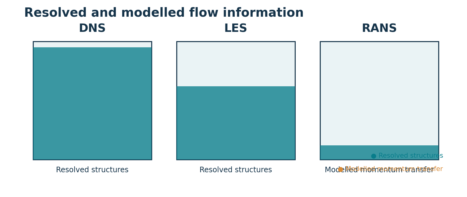
2. DNS, LES and RANS are different descriptions
| Approach | Representation | Use in this guide |
|---|---|---|
| DNS | Resolves all relevant turbulence scales | Conceptual reference only; computationally demanding |
| LES | Resolves large turbulent structures and models subgrid scales | Introduction only; requires its own mesh/time validation |
| RANS | Resolves mean fields and closes turbulence correlations | Main focus |
Steady RANS models a mean flow, not a time-resolved eddy movie. An unsteady RANS (URANS) simulation is possible, but does not become an LES simply by setting a transient time scheme. The Reynolds stress term introduced by time or ensemble averaging is approximated by the closure. Most common industrial two-equation models rely on an eddy-viscosity hypothesis and generate the turbulent kinematic viscosity field nut.
This assumption is useful but limited in strongly anisotropic, curved, rotating and separated flows. An attractive streamline visualization is not a substitute for a quantified benchmark.
Deep dive · What a DNS of this step would cost
For a DNS the ratio between the largest scale and the Kolmogorov scale grows as Re^(3/4) in each direction, so the number of 3D points grows as Re^(9/4). With Re ≈ 2.5·10⁴:
N_DNS ~ Re^(9/4) = 25400^2.25 ≈ 8·10⁹ points (order of magnitude)
N_RANS 2D (pitzDaily) ≈ 1·10⁴ cells
ratio ≈ 10⁶
Moreover DNS is necessarily three-dimensional and transient, with thousands of time steps to obtain converged statistics, whereas steady RANS converges in a few thousand iterations on a 2D mesh. LES sits in between: it resolves the large eddies, but near walls the cost again grows rapidly with Re if the boundary layer is resolved. This gap of six or more orders of magnitude is what makes RANS the everyday tool of engineering, with the limits the guide highlights.
Deep dive · URANS, LES and the role of the mesh
- Steady RANS: the mesh must resolve mean-field gradients; refining it improves the solution of the RANS equations, but does not bring the result closer to real turbulence beyond what the model allows;
- URANS: represents only large-scale instabilities clearly separated from the turbulent spectrum (for example periodic shedding); turbulent fluctuations remain modelled by ν_t;
- LES: the filter size is tied to the mesh, so the mesh is part of the model; a spatial convergence study has a different meaning than in RANS and requires time statistics.
3. Official Foundation 14 case: pitzDailySteady
The exercise is built around $FOAM_TUTORIALS/incompressibleFluid/pitzDailySteady, a steady backward-facing-step case included with OpenFOAM Foundation 14. The sudden enlargement creates flow separation and downstream reattachment, offering a meaningful setting for comparing turbulence closures. The official case already includes 0/k, 0/epsilon, 0/omega and 0/nut.
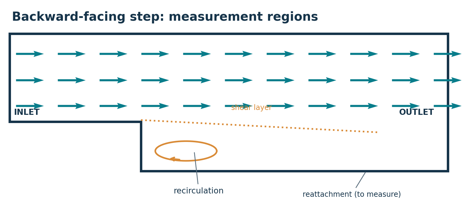
The supplied settings include an inlet U = (10, 0, 0) m/s, kinematic viscosity ν = 1×10⁻⁵ m²/s, zero kinematic-pressure reference at the outlet, and no-slip walls. The computational configuration is quasi-two-dimensional with empty front/back patches. kEpsilon is the original turbulence model.
Mesh generation uses the official resources/blockMesh/pitzDaily dictionary. It is intentionally supplied outside the case folder. The blockMesh -dict ... invocation reproduced in the scripts follows the official tutorial run sequence.
Scientific limitation: the exercise is a controlled methodological comparison, not experimental validation of a backward-facing step. We do not claim any drag, reattachment or pressure measurements before running the actual cases.
Deep dive · The pitzDaily geometry and the experimental reference
The case is named after the Pitz and Daily (1983) experiment on a turbulent mixing layer downstream of a rearward-facing step. The dimensions can be read directly from the resource dictionary:
D="$FOAM_TUTORIALS/resources/blockMesh/pitzDaily"
foamDictionary "$D" -entry convertToMeters
foamDictionary "$D" -entry vertices
foamDictionary "$D" -entry blocks
From the vertex coordinates you obtain the inlet-channel height, the step height and the expansion ratio, which should be recorded in the project notebook before any comparison. In the literature on steps with an expansion ratio around 2 and Re of order 10⁴ the measured reattachment length is typically a few step heights (of order 6–8 h), and standard k-ε is known to tend to underpredict it because it produces too much turbulent viscosity in the shear layer. Use these values as an order of magnitude to recognise an anomalous result, not as validation data: a real comparison needs the original measurements and the same inlet conditions.
Practical tip · Read the tutorial the way the distribution runs it
T="$FOAM_TUTORIALS/incompressibleFluid/pitzDailySteady"
cat "$T/Allrun"
ls "$T" "$T/0" "$T/constant" "$T/system"
foamDictionary "$T/system/fvSolution" -entry SIMPLE
foamDictionary "$T/system/controlDict" -entry endTime
foamDictionary "$T/0/U" -entry boundaryField
The official Allrun is the source of truth for the commands: if a new version changes the sequence (for example the mesh resource path), the guide’s script must be adapted to it, not the other way round. The SIMPLE block shows the stopping criteria (residualControl) with which the solver declares convergence.
4. Select the model in constant/momentumTransport
OpenFOAM Foundation 14 uses the following model-selection structure:
simulationType RAS;

RAS
{
    model       kEpsilon;
    turbulence  on;
}
For the second run, replace only model kEpsilon; with model kOmegaSST;. Do not simultaneously change inlet velocity, mesh, physical properties or discretization schemes; that would prevent isolating the turbulence model as a variable.
The two-equation k-ε family is widely used in industrial internal flows; k-ω SST blends k-ω and k-ε formulations and is commonly used when boundary layers and separation matter. Neither is universally the “most accurate” model. The model choice must be supported by evidence for the particular configuration.
Optional refresher — RANS variables. k: turbulent kinetic energy per unit mass [m²/s²]. epsilon: dissipation rate [m²/s³]. omega: specific dissipation [s⁻¹]. nut: turbulent kinematic viscosity [m²/s]. The 0/ files are OpenFOAM field specifications, not general-purpose text parameters.
Deep dive · The equations of the two models in brief
| Aspect | k-ε (Launder–Spalding) | k-ω SST (Menter) |
|---|---|---|
| transported variables | k, ε | k, ω |
| turbulent viscosity | ν_t = Cμ k² / ε | ν_t = a₁ k / max(a₁ ω, S F₂) |
| typical constants | Cμ = 0.09 · C₁ = 1.44 · C₂ = 1.92 · σ_k = 1.0 · σ_ε = 1.3 | a₁ = 0.31 + k-ω and k-ε coefficients blended by F₁ |
| near the wall | needs wall functions; not integrable to the wall in standard form | ω formulation near the wall, k-ε away from it |
| adverse pressure gradient | tends to overpredict ν_t and delay/reduce separation | the limiter with F₂ reduces ν_t where production exceeds dissipation |
The ν_t limiter is the difference that matters most in this case: in the shear layer starting from the step edge k-ε produces high turbulent viscosity, which mixes rapidly and shortens the recirculation bubble; SST limits it and tends to produce longer bubbles. The coefficients actually used are printed at the start of log.foamRun (block kEpsilonCoeffs or kOmegaSSTCoeffs): keep them as part of the run documentation.
Practical tip · Prove that only the model changed
R="$HOME/OpenFOAM/guide09_run01"
diff -ru "$R/kEpsilon" "$R/kOmegaSST"
foamDictionary "$R/kEpsilon/constant/momentumTransport" -entry RAS/model
foamDictionary "$R/kOmegaSST/constant/momentumTransport" -entry RAS/model
Before launching, the diff must show only the model line and the GUIDE09_MODEL.txt file. Save the output in a campaign file (diff -ru ... > diff_before_run.txt): it is the documentary proof that the comparison is controlled.
5. Keep turbulence inlet conditions consistent
An approximate inlet specification can be derived from mean inlet speed U, turbulence intensity I and an assumed turbulent length scale ℓ:
k       = 1.5 × (U I)²
epsilon = Cmu^(3/4) × k^(3/2) / ℓ
omega   = sqrt(k) / (Cmu^(1/4) × ℓ)
Cmu     = 0.09  (usual estimate)
For U = 10 m/s, I = 0.05 and ℓ = 0.00254 m, this gives approximately k = 0.375 m²/s², epsilon = 14.86 m²/s³, omega = 440 s⁻¹. These are close to the original tutorial values. This consistency is not proof that actual experimental inlet turbulence is known; it is a controlled assumption.
python3 scripts/estimate_inlet.py --U 10 --I 0.05 --L 0.00254Inspect both the initial field and the inlet boundary condition in 0/k, 0/epsilon and 0/omega. Ensure the fields required by the chosen closure exist. A second exercise may vary turbulence intensity or length scale, but must keep those changes separate from the model-comparison campaign.
Deep dive · The estimate_inlet.py script and a consistency check on ν_t
#!/usr/bin/env python3
# SPDX-License-Identifier: GPL-3.0-or-later
"""Calculate indicative RANS inlet k/epsilon/omega from U, intensity and length scale."""
import argparse
from math import sqrt


def estimates(U, intensity, length, cmu=0.09):
    if not (U > 0 and 0 < intensity < 1 and length > 0 and cmu > 0):
        raise ValueError("U>0, 0<I<1, length>0 and Cmu>0 are required")
    k = 1.5 * (U * intensity)**2
    epsilon = cmu**0.75 * k**1.5 / length
    omega = sqrt(k) / (cmu**0.25 * length)
    return k, epsilon, omega


def main():
    p = argparse.ArgumentParser(description=__doc__)
    p.add_argument("--U", type=float, default=10.0, help="Mean inlet speed in m/s")
    p.add_argument("--I", type=float, default=0.05, help="Turbulence intensity as a fraction")
    p.add_argument("--L", type=float, default=0.00254, help="Turbulence length scale in m")
    a = p.parse_args()
    try:
        k, epsilon, omega = estimates(a.U, a.I, a.L)
    except ValueError as ex:
        p.error(str(ex))
    print(f"k       = {k:.8g} m2/s2")
    print(f"epsilon = {epsilon:.8g} m2/s3")
    print(f"omega   = {omega:.8g} 1/s")
    print("Indicative estimates; verify consistency with the selected model and experiment.")

if __name__ == "__main__":
    main()
$ python3 scripts/estimate_inlet.py --U 10 --I 0.05 --L 0.00254
k = 0.375 m2/s2
epsilon = 14.855767 m2/s3
omega = 440.17086 1/s
Indicative estimates; verify consistency with the selected model and experiment.The three relations are built so that both models start from the same turbulent viscosity: ν_t = Cμ k²/ε = 0.09 · 0.375² / 14.856 ≈ 8.52·10⁻⁴ m²/s and ν_t = k/ω = 0.375 / 440.17 ≈ 8.52·10⁻⁴ m²/s. This is the check to make every time the inlet values are changed: if the two ν_t differ, the two models start from different conditions and the comparison is no longer controlled.
Deep dive · Sensitivity to the inlet assumptions
| Change | k | ε | ω | ν_t |
|---|---|---|---|---|
| I doubled | × 4 | × 8 | × 2 | × 2 |
| ℓ doubled | = | × ½ | × ½ | × 2 |
| U doubled | × 4 | × 8 | × 2 | × 2 |
The length ℓ = 2.54 mm corresponds to 10 % of the inlet-channel height; a widespread rule of thumb is ℓ ≈ 0.07 Dₕ, which with Dₕ = 50.8 mm would give 3.6 mm. Neither is “right”: they are assumptions. Since inlet ν_t changes proportionally with I and ℓ, a sensitivity campaign on these two parameters (separate from the model comparison, as the guide requires) tells you how much reattachment depends on information usually not known precisely.
6. Near-wall modelling and the meaning of y+
The dimensionless wall coordinate y⁺ = y uτ / ν, where uτ = √(τw/ρ), measures the first-cell centre distance scaled by the local viscous length. It is a diagnostic for whether the mesh is consistent with the selected wall treatment, not a universal mesh-quality grade.
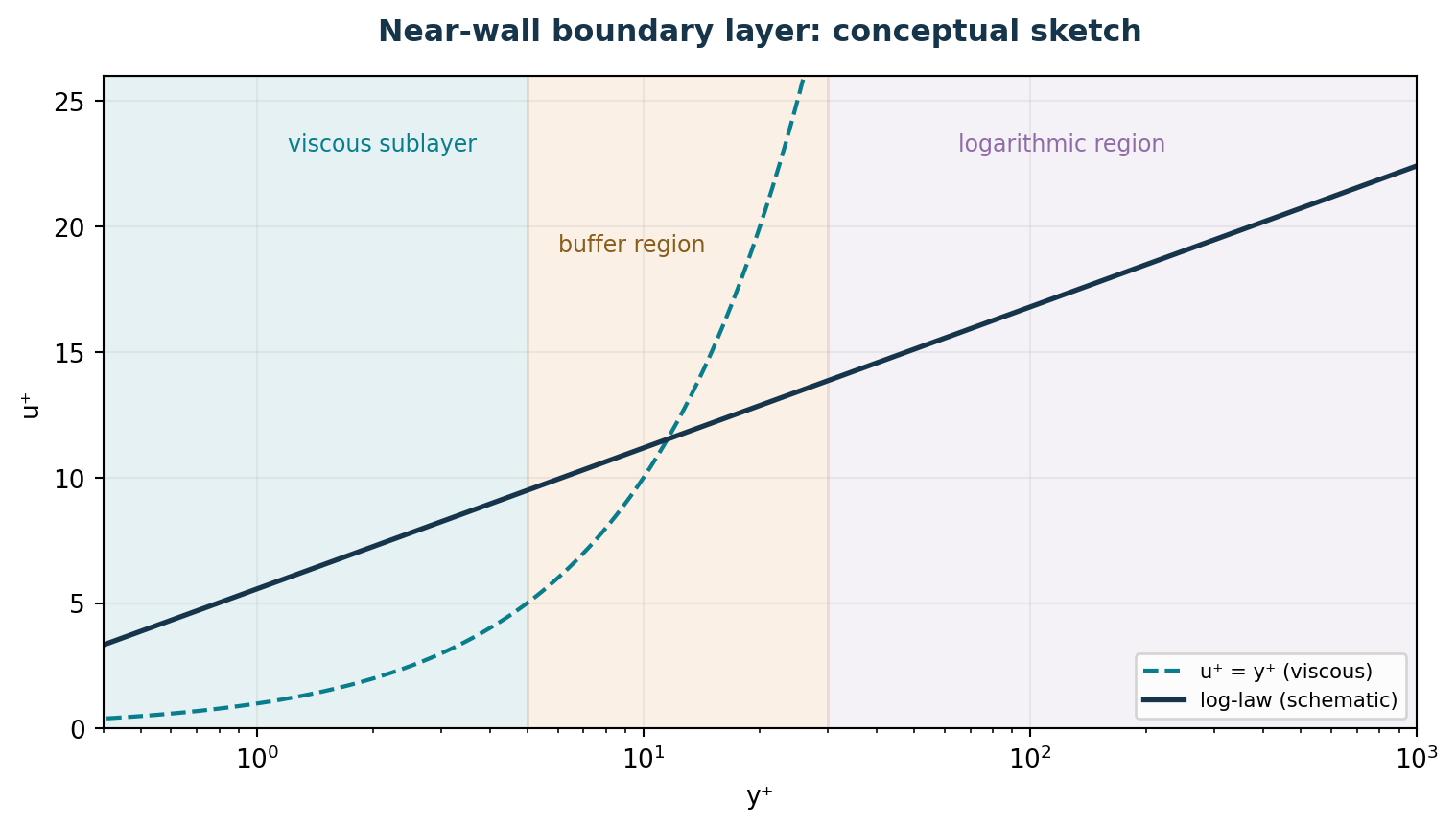
In broad terms, y⁺ around 1 is a common target for resolving the viscous sublayer. Conventional high-Re log-law wall functions often target y⁺ roughly 30–300. These are not universal pass/fail thresholds: blending, specific wall functions, wall curvature, separation and roughness alter the appropriate range. The buffer layer deserves attention, but its mere presence does not automatically invalidate a model with suitable blending.
In the official case, 0/U uses noSlip for upperWall and lowerWall; 0/k uses kqRWallFunction; 0/nut uses nutkWallFunction; 0/epsilon uses epsilonWallFunction; and 0/omega uses omegaWallFunction. frontAndBack uses empty throughout the nominally 2D formulation.
Optional refresher — First-cell height. A design estimate for the first-layer height requires an estimate of friction velocity uτ, which is not known precisely before simulation. Start from an engineering estimate, simulate, evaluate y⁺ on the actual walls, then design a new mesh campaign. Do not claim a particular y⁺ merely because a spacing was entered in a mesh dictionary.
Deep dive · Estimating y⁺ before the run: a numerical example
For the inlet channel, upstream of the step, Dean’s correlation for turbulent plane-channel flow can be used, Cf = 0.073 Re^(−1/4) with Re based on the channel height. The following script, added to this guide, standard library only, applies the estimate:
#!/usr/bin/env python3
"""A-priori estimate of y+ for the first cell centre in a plane channel (engineering estimate).

Uses Dean's correlation Cf = 0.073 Re^-1/4 (Re on full channel height and bulk velocity),
valid roughly for 6e3 < Re < 6e5 in smooth, fully developed channel flow.
Usage: first_cell.py --U 10 --H 0.0254 --nu 1e-5 [--yp 0.25e-3 0.5e-3 1e-3] [--target 1 30 100]
Standard library only. License: GNU GPL v3 or later.
"""
from __future__ import annotations
import argparse, math


def main() -> None:
    ap = argparse.ArgumentParser(description=__doc__, formatter_class=argparse.RawDescriptionHelpFormatter)
    ap.add_argument("--U", type=float, required=True, help="bulk velocity [m/s]")
    ap.add_argument("--H", type=float, required=True, help="full channel height [m]")
    ap.add_argument("--nu", type=float, required=True, help="kinematic viscosity [m2/s]")
    ap.add_argument("--yp", type=float, nargs="*", default=[], help="first-cell-centre distances [m]")
    ap.add_argument("--target", type=float, nargs="*", default=[1.0, 30.0, 100.0], help="target y+ values")
    a = ap.parse_args()
    Re = a.U * a.H / a.nu
    Cf = 0.073 * Re ** -0.25
    utau = a.U * math.sqrt(Cf / 2.0)
    lv = a.nu / utau
    print(f"Re_H = {Re:.4g}   Cf = {Cf:.4g}   u_tau = {utau:.4g} m/s   viscous length nu/u_tau = {lv:.4g} m")
    if not 6e3 <= Re <= 6e5:
        print("warning: Re outside the usual range of Dean's correlation")
    for y in a.yp:
        print(f"y_P = {y:.4g} m  ->  y+ = {y / lv:.4g}   (first cell height ~ {2 * y:.4g} m)")
    for t in a.target:
        print(f"target y+ = {t:g}  ->  y_P = {t * lv:.4g} m  (first cell height ~ {2 * t * lv:.4g} m)")
    print("Estimate only: separated and reattaching regions have very different wall shear; measure y+ after the run.")


if __name__ == "__main__":
    main()
$ python3 first_cell.py --U 10 --H 0.0254 --nu 1e-5 --yp 0.25e-3 0.5e-3 1e-3
Re_H = 2.54e+04 Cf = 0.005782 u_tau = 0.5377 m/s viscous length nu/u_tau = 1.86e-05 m
y_P = 0.00025 m -> y+ = 13.44 (first cell height ~ 0.0005 m)
y_P = 0.0005 m -> y+ = 26.89 (first cell height ~ 0.001 m)
y_P = 0.001 m -> y+ = 53.77 (first cell height ~ 0.002 m)
target y+ = 1 -> y_P = 1.86e-05 m (first cell height ~ 3.72e-05 m)
target y+ = 30 -> y_P = 0.0005579 m (first cell height ~ 0.001116 m)
target y+ = 100 -> y_P = 0.00186 m (first cell height ~ 0.00372 m)The viscous length is about 19 μm: resolving the viscous sublayer (y⁺ ≈ 1) would need a first cell of about 37 μm, log-law wall functions (y⁺ ≈ 30) about 1.1 mm. Downstream of the step the estimate does not hold: inside the bubble the wall shear passes through zero, so y⁺ tends to zero near the separation and reattachment points whatever the mesh. That is why the guide asks to look at the distribution, not at a single value.
Deep dive · What wall functions do in OpenFOAM
nutkWallFunction: in the wall cell it computes ν_t from k so that wall shear follows the log law when y⁺ exceeds a threshold (of order 11, where the linear and log laws meet); below the threshold only molecular viscosity acts;epsilonWallFunctionandomegaWallFunction: impose ε or ω in the wall cell according to the log-region scale (ω also according to the viscous one, blending the two in recent versions);kqRWallFunction: zero gradient of k at the wall, consistent with the functions above.
Details (thresholds, blended formulations) change between versions: the reference is the source code of your installation, browsable in the C++ documentation cited in the sources. The operational consequence remains: y⁺ must be compared with the validity range of the wall function actually chosen.
Practical tip · List the wall conditions of all fields
cd "$HOME/OpenFOAM/guide09_run01/kOmegaSST"
for f in U p k epsilon omega nut; do
  printf "%-8s lowerWall: %s\n" "$f" "$(foamDictionary 0/$f -entry boundaryField/lowerWall/type -value)"
done
A table like this, saved in the case folder, immediately shows a frequent error: a field with the wrong or missing condition on a patch. Repeat it for upperWall, inlet and outlet.
7. Prepare two independent cases from Windows
Connect from Windows PowerShell to the Linux server using SSH, load OpenFOAM 14 and transfer the scripts/ folder using FileZilla. Use Notepad++ for optional local edits, keeping line endings as LF. The preparation script creates new case directories and refuses to overwrite existing work.
foamVersion
echo "$FOAM_TUTORIALS"
python3 scripts/prepare_cases.py --out "$HOME/OpenFOAM/guide09_run01"
ls "$HOME/OpenFOAM/guide09_run01/kEpsilon"
ls "$HOME/OpenFOAM/guide09_run01/kOmegaSST"
Both cases are independent copies of the official tutorial. The only intended modelling change between them is model kEpsilon; versus model kOmegaSST; in constant/momentumTransport. The script verifies the original model selector before changing anything and rejects an existing destination folder.
The original tutorial files are never modified. Retain the unmodified comparison dataset before planning further mesh, turbulence-intensity or boundary-condition studies.
Deep dive · The prepare_cases.py script, full text and commentary
#!/usr/bin/env python3
# SPDX-License-Identifier: GPL-3.0-or-later
"""Prepare isolated OpenFOAM Foundation 14 pitzDailySteady RANS cases."""
import argparse
import csv
import os
from pathlib import Path
import shutil
import sys

MODELS = {"kEpsilon": "kEpsilon", "kOmegaSST": "kOmegaSST"}


def prepare(template: Path, output: Path):
    template = template.expanduser().resolve(strict=True)
    output = output.expanduser().resolve()
    if not template.is_dir():
        raise ValueError("Tutorial template is not a directory")
    for required in ("0/U", "0/k", "0/epsilon", "0/omega", "0/nut",
                     "system/controlDict", "system/fvSchemes", "system/fvSolution",
                     "constant/momentumTransport", "constant/physicalProperties"):
        if not (template / required).is_file():
            raise ValueError(f"Missing tutorial file: {required}")
    if output.exists():
        raise FileExistsError(f"Destination exists (will not overwrite): {output}")
    if output == template or template in output.parents and output == template:
        raise ValueError("Output cannot be the template")
    output.mkdir(parents=True, exist_ok=False)
    try:
        for case_name, model in MODELS.items():
            dst = output / case_name
            shutil.copytree(template, dst, symlinks=False,
                            ignore=shutil.ignore_patterns("processor*", "log.*", "postProcessing"))
            path = dst / "constant/momentumTransport"
            text = path.read_text(encoding="utf-8")
            import re
            if len(re.findall(r"(?m)^\s*model\s+kEpsilon\s*;", text)) != 1:
                raise ValueError("Expected exactly one 'model kEpsilon;' in tutorial momentumTransport")
            text = re.sub(r"(?m)^(\s*model\s+)kEpsilon(\s*;)",
                          lambda m: m.group(1) + model + m.group(2), text, count=1)
            path.write_text(text, encoding="utf-8", newline="\n")
            (dst / "GUIDE09_MODEL.txt").write_text(
                f"model={model}\nsource={template}\n"+
                "Run independently; no experimental validation is implied.\n", encoding="utf-8")
        with (output / "cases.csv").open("w", encoding="utf-8", newline="") as f:
            writer = csv.writer(f)
            writer.writerow(["case", "model", "mesh", "status"])
            for name, model in MODELS.items():
                writer.writerow([name, model, "pitzDaily tutorial resource", "not_run"])
    except Exception:
        # Only clean up the new directory created by this function, never pre-existing work.
        shutil.rmtree(output)
        raise
    print(f"Created two independent cases at {output}")


def main():
    parser = argparse.ArgumentParser(description=__doc__)
    parser.add_argument("--out", type=Path, required=True)
    parser.add_argument("--template", type=Path,
                        default=Path(os.environ.get("FOAM_TUTORIALS", "")) / "incompressibleFluid/pitzDailySteady")
    args = parser.parse_args()
    if not os.environ.get("FOAM_TUTORIALS") and "--template" not in sys.argv:
        parser.error("FOAM_TUTORIALS is not set; load OpenFOAM 14 or provide --template")
    try:
        prepare(args.template, args.out)
    except (FileNotFoundError, FileExistsError, ValueError, OSError) as exc:
        parser.exit(2, f"Preparation failed: {exc}\n")

if __name__ == "__main__":
main()- checks that every file needed for the comparison exists in the tutorial before creating anything;
- requires exactly one
model kEpsilon;line: should a future tutorial change, the script stops instead of producing a wrong comparison; - on error it removes only the folder it has just created itself, never pre-existing work, because an existing destination is refused at the start;
- writes
cases.csvwith statusnot_run: a minimal campaign register to be updated by hand.
8. Execute each model without replacing existing logs
For a long job, use tmux so a lost SSH connection does not interrupt the detached terminal session:
tmux new -s guide09
chmod +x scripts/run_case.sh
scripts/run_case.sh "$HOME/OpenFOAM/guide09_run01/kEpsilon"
scripts/run_case.sh "$HOME/OpenFOAM/guide09_run01/kOmegaSST"
For each case, run_case.sh executes blockMesh -dict "$FOAM_TUTORIALS/resources/blockMesh/pitzDaily", checkMesh, and foamRun, followed by an attempt at foamPostProcess -solver incompressibleFluid -func yPlus -latestTime. Output files are log.blockMesh, log.checkMesh, log.foamRun and log.yPlus.
If a log or mesh already exists, the runner refuses to continue. It is intentionally not an automatic restart or cleanup tool. A partially failed case should be inspected and resumed through a separately documented recovery procedure, with the original outputs preserved.
tail -n 60 "$HOME/OpenFOAM/guide09_run01/kOmegaSST/log.foamRun"Deep dive · The run_case.sh script, full text and commentary
#!/usr/bin/env bash
# SPDX-License-Identifier: GPL-3.0-or-later
# Run one untouched pitzDailySteady-derived case, without overwriting logs/results.
set -Eeuo pipefail
if [[ $# -ne 1 ]]; then
  echo "Usage: $0 /absolute/path/to/prepared/case" >&2
  exit 2
fi
: "${FOAM_TUTORIALS:?Source OpenFOAM 14 environment before running}"
case_dir="$(realpath "$1")"
[[ -f "$case_dir/GUIDE09_MODEL.txt" ]] || { echo "Not a Guide 09 prepared case" >&2; exit 2; }
[[ -f "$FOAM_TUTORIALS/resources/blockMesh/pitzDaily" ]] || { echo "Missing OpenFOAM tutorial mesh resource" >&2; exit 2; }
for logfile in log.blockMesh log.checkMesh log.foamRun log.yPlus; do
  [[ ! -e "$case_dir/$logfile" ]] || { echo "Existing $logfile: refusing to overwrite" >&2; exit 2; }
done
[[ ! -d "$case_dir/constant/polyMesh" ]] || { echo "Existing mesh: refusing to alter case" >&2; exit 2; }
cd "$case_dir"
echo "Running case: $case_dir"
blockMesh -dict "$FOAM_TUTORIALS/resources/blockMesh/pitzDaily" > log.blockMesh 2>&1
checkMesh > log.checkMesh 2>&1
foamRun > log.foamRun 2>&1
# Failure in optional yPlus post-processing does not invalidate a finished flow solution.
if ! foamPostProcess -solver incompressibleFluid -func yPlus -latestTime > log.yPlus 2>&1; then
  echo "WARNING: yPlus post-processing failed; see log.yPlus" >&2
fi
echo "Completed flow solution for $case_dir"
The check on constant/polyMesh is an important protection: re-running blockMesh on an already computed case would replace the mesh, leaving incompatible saved fields. The y⁺ post-processing is separated from the run with if !: an error in it produces a warning but neither deletes nor invalidates the flow solution.
Deep dive · Reading the log of a steady run
- in a steady run
Time = ...is an iteration counter, not physical time; - if
residualControlis active, the solver stops beforeendTimewith a message such as “SIMPLE solution converged in N iterations”: record N for each model; bounding k,bounding epsilonorbounding omegalines mean negative values clipped to a minimum: a few in the first iterations are common, persisting to the end they signal a mesh, condition or scheme problem;- continuity errors
sum localthat do not decrease indicate a non-converged solution even if residuals look low.
grep -E "converged in|^End" log.foamRun
grep -c "^bounding" log.foamRun
grep "bounding" log.foamRun | tail -3
Practical tip · Two runs in parallel, if the server allows
The two cases are independent: with at least two free cores they can be launched in two separate tmux windows (Ctrl+b then c for a new window). On a 2D mesh of about ten thousand cells each run uses one core and little memory; total time halves with no risk to the data, because the folders are separate. Check the load first with uptime or htop if the server is shared.
9. Calculate and assess y+ rather than guessing it
In Foundation 14, the appropriate post-processing utility is foamPostProcess. Our command includes -solver incompressibleFluid to load the model context for turbulent wall quantities. -func yPlus selects the function object, and -latestTime selects the most recent saved solution time. Check log.yPlus for success and locate the written yPlus field.
cd "$HOME/OpenFOAM/guide09_run01/kOmegaSST"
tail -n 30 log.yPlus
find . -type f -name 'yPlus' | head
An unsuccessful y+ post-processing attempt does not automatically mean that the flow solver failed, but it means near-wall adequacy has not been demonstrated. A y+ file alone is also not evidence of adequacy: inspect its distribution, extremes, wall patches and critical regions, particularly close to the step and reattachment region.
Deep dive · Where y⁺ ends up and how to read its numbers
The yPlus function object writes the yPlus field into the last saved time folder and prints in the log a per-wall-patch summary with minimum, maximum and average. The summary is the first thing to look at:
grep -i "y+" log.yPlus
foamListTimes -latestTime
ls "$(foamListTimes -latestTime)"
An acceptable average with a minimum near zero and a very high maximum is not contradictory: in the recirculation bubble wall shear is small, under the inlet shear layer it is large. The assessment must be made by zones: inlet channel, region behind the step, reattachment zone, upper wall.
Deep dive · Wall shear stress: the quantity for reattachment
The same post-processing mechanism computes wall shear stress, which is needed to define reattachment reproducibly (section 11). Before using it, check the name of the function available in your installation:
foamPostProcess -list | grep -i -E "wallShear|yPlus"
foamPostProcess -solver incompressibleFluid -func wallShearStress -latestTime > log.wallShearStress 2>&1
tail -n 20 log.wallShearStress
The resulting field is per unit density [m²/s²] and has three components: for reattachment the component parallel to the lower wall matters, that is x in this geometry. This command also writes a separate log and does not modify the flow fields.
10. Quantitative analysis on Windows using ParaView
Connect ParaView on Windows to Linux pvserver as described in Guide 1, and load each case separately. Use matching geometrical positions, physical units and the same colour-scale limits. Independent automatic colour scales can make similar fields look misleadingly different.
Examine velocity U, kinematic pressure p, turbulent viscosity nut, a downstream velocity profile, and negative streamwise-velocity regions. Plot Over Line supports reproducible velocity profiles; Calculator and Threshold can help select backflow, provided you record exactly what expression and criterion were used. A rigorous reattachment estimate requires a stated physical definition, typically linked to the sign of wall shear stress, rather than visual inspection of streamline shapes alone.
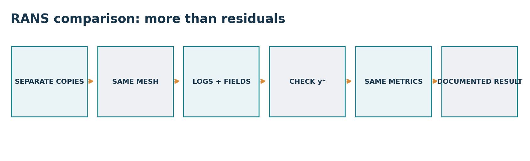
Before assigning differences to the closure, confirm that the chosen wall treatment and measured y+ are suitable in both cases. When exporting a CSV, document the filter, sample coordinates, number of samples and interpolation behaviour.
Deep dive · Measuring reattachment with an explicit criterion
- in ParaView apply Extract Block and select only the
lowerWallpatch (withwallShearStressamong the loaded fields); - with a 2D one-cell-thick geometry the patch is a strip: Plot Data or Plot Over Line along x at constant z give the x component versus position;
- export to CSV with File → Save Data and compute the sign changes with the following script, added to this guide.
#!/usr/bin/env python3
"""Find wall-shear sign changes along a wall from a ParaView CSV export.

The CSV must contain a coordinate column (default 'Points:0') and the streamwise
wall-shear component (default 'wallShearStress:0'). Rows are sorted by coordinate;
each sign change is located by linear interpolation between neighbouring samples.
Values are per unit density [m2/s2] in incompressible OpenFOAM. Establish the sign
convention from a region where the flow is certainly attached (far downstream)
before naming a crossing 'separation' or 'reattachment'.
Usage: find_reattachment.py lowerWall.csv [--x Points:0] [--tau wallShearStress:0]
       [--xmin 0] [--h 0.0254]
Standard library only. License: GNU GPL v3 or later.
"""
from __future__ import annotations
import argparse, csv
from pathlib import Path


def main() -> None:
    ap = argparse.ArgumentParser(description=__doc__, formatter_class=argparse.RawDescriptionHelpFormatter)
    ap.add_argument("csv", type=Path)
    ap.add_argument("--x", default="Points:0", help="coordinate column")
    ap.add_argument("--tau", default="wallShearStress:0", help="streamwise wall shear column")
    ap.add_argument("--xmin", type=float, default=float("-inf"), help="ignore samples upstream of this x")
    ap.add_argument("--h", type=float, default=None, help="step height for x/h output")
    a = ap.parse_args()
    with a.csv.open(newline="", encoding="utf-8") as f:
        rd = csv.DictReader(f)
        for col in (a.x, a.tau):
            if col not in (rd.fieldnames or []):
                ap.error(f"column '{col}' not found; available: {rd.fieldnames}")
        pts = sorted((float(r[a.x]), float(r[a.tau])) for r in rd if float(r[a.x]) >= a.xmin)
    if len(pts) < 2:
        ap.error("not enough samples")
    found = 0
    for (x0, t0), (x1, t1) in zip(pts, pts[1:]):
        if t0 == 0 or t0 * t1 < 0:
            xc = x0 if t0 == 0 else x0 + (x1 - x0) * (-t0) / (t1 - t0)
            kind = "negative -> positive" if t1 > t0 else "positive -> negative"
            extra = f"   x/h = {xc / a.h:.4g}" if a.h else ""
            print(f"sign change at x = {xc:.6g} m ({kind}){extra}")
            found += 1
    print(f"{len(pts)} samples, {found} sign change(s). Report the criterion and the wall patch used.")


if __name__ == "__main__":
    main()
Tested on a synthetic profile with a known sign change at x = 0.17 m, the script returns:
$ python3 find_reattachment.py test_wall.csv --xmin 0.001 --h 0.0254
sign change at x = 0.17 m (negative -> positive)   x/h = 6.693
200 samples, 1 sign change(s). Report the criterion and the wall patch used.
More than one sign change is normal: near the step corner a small counter-rotating secondary bubble may exist. Report all points found and state which one you take as main reattachment, and why.
Practical tip · Quantifying the recirculation bubble
Besides its length, the bubble has a measurable area. In ParaView: Threshold on U_X with upper bound 0 (cells with backflow), then Integrate Variables: the integrated volume divided by the domain thickness in z gives the in-plane bubble area. Done with the same filter on both cases, it is an extra indicator, insensitive to a single sampling point. Always state the criterion (U_x < 0, not “blue zone of the colour map”).
11. Pressure and physically meaningful comparisons
The incompressible p field in Foundation 14 represents kinematic pressure [m²/s²]. For a constant-density fluid, physical pressure differences in pascals are ΔP = ρ Δp. Merely relabelling a ParaView axis is not a conversion.
A pressure-drop comparison must use exactly defined upstream/downstream sections and an explicit averaging operation. Likewise, a reattachment-length comparison must define its measurement criterion consistently across models. The end of a streamline swirl is not automatically a wall-shear sign change.
Deep dive · From kinematic pressure to pascals: orders of magnitude
| Assumed fluid | ρ [kg/m³] | ½ρU² with U = 10 m/s | 1 m²/s² of kinematic p |
|---|---|---|---|
| air (≈ 20 °C) | 1.2 | 60 Pa | 1.2 Pa |
| water (≈ 20 °C) | 998 | 49.9 kPa | 998 Pa |
In kinematic units the reference dynamic pressure is ½U² = 50 m²/s² whatever the fluid; the value in pascals depends entirely on the declared density. Note that ν = 1·10⁻⁵ m²/s corresponds exactly neither to air (about 1.5·10⁻⁵) nor to water (about 1·10⁻⁶): it is a tutorial value. This is why density must be declared as an assumption of the measurement, and a ΔP in pascals only makes sense together with it.
Deep dive · Reproducible section averages with post-processing
For inlet and outlet, which are patches, averages can be computed without ParaView using the predefined foamPostProcess configurations. Names and arguments depend on the version: list them and read the configuration file header before using them.
foamPostProcess -list | grep -i -E "patch|surface"
# example to adapt to what is listed
foamPostProcess -solver incompressibleFluid -func "patchAverage(name=inlet, p)" -latestTime
foamPostProcess -solver incompressibleFluid -func "patchAverage(name=outlet, p)" -latestTime
foamPostProcess -solver incompressibleFluid -func "patchFlowRate(patch=outlet)" -latestTime
The result goes to postProcessing/ with one file per function: the difference of the two averages, multiplied by the declared density, is the ΔP between inlet and outlet. For internal sections (for example at x = 0.2 m) you need a sampling plane or Slice + Integrate Variables in ParaView, with area-weighted averaging.
12. Summarise logs and measured observables separately
The supplied collect_logs.py extracts the last available initial residual for recognised fields, reports whether log.foamRun exists and checks for the terminal End marker. It does not invent y+, pressure loss, flow rate or reattachment distance; those must be obtained from actual numerical results and placed in measurement_template.csv.
python3 scripts/collect_logs.py "$HOME/OpenFOAM/guide09_run01" \
--output "$HOME/OpenFOAM/guide09_run01_log_summary.csv"| Quantity | k-ε | k-ω SST | Evidence required |
|---|---|---|---|
| Solver completion | To measure | To measure | Logs, convergence, conservation |
| Wall y⁺ | To measure | To measure | foamPostProcess and ParaView |
| Pressure loss [Pa] | To measure | To measure | Same sections, declared density |
| Reattachment length [m] | To measure | To measure | Explicit wall-based criterion |
| Streamwise velocity profiles | To measure | To measure | Identical Plot Over Line coordinates |
Smaller residuals do not necessarily imply greater physical accuracy. If the flow is inherently unsteady, a steady RANS model may produce oscillations or fail to converge. Do not suppress physically meaningful behaviour solely to obtain a smoother residual plot.
Deep dive · The collect_logs.py script and the measurement sheet template
#!/usr/bin/env python3
# SPDX-License-Identifier: GPL-3.0-or-later
"""Collect traceable last residuals from Guide 09 solver logs (no invented CFD values)."""
import argparse
import csv
from pathlib import Path
import re

RESIDUAL = re.compile(
    r"Solving\s+for\s+([A-Za-z0-9_]+)\s*,\s*Initial residual\s*=\s*"
    r"([+\-0-9.eE]+)\s*,\s*Final residual\s*=\s*([+\-0-9.eE]+)"
)
FIELDS = ("p", "Ux", "Uy", "Uz", "k", "epsilon", "omega")

def summarize(case: Path):
    log = case / "log.foamRun"
    result = {"case": case.name, "model": "", "log_present": str(log.is_file()),
              "end_marker": "", "residual_records": 0}
    for f in FIELDS:
        result[f + "_initial_residual_last"] = ""
    info = case / "GUIDE09_MODEL.txt"
    if info.is_file():
        for line in info.read_text(encoding="utf-8").splitlines():
            if line.startswith("model="):
                result["model"] = line.split("=", 1)[1]
    if log.is_file():
        content = log.read_text(encoding="utf-8", errors="replace")
        result["end_marker"] = str(bool(re.search(r"(?m)^End\s*$", content)))
        for field, initial, final in RESIDUAL.findall(content):
            result["residual_records"] += 1
            key = field + "_initial_residual_last"
            if key in result:
                result[key] = initial
    return result

def main():
    p = argparse.ArgumentParser(description=__doc__)
    p.add_argument("root", type=Path)
    p.add_argument("--output", type=Path, default=Path("summary_log.csv"))
    a = p.parse_args()
    root = a.root.expanduser().resolve()
    cases = [root / name for name in ("kEpsilon", "kOmegaSST")]
    records = [summarize(c) for c in cases]
    if a.output.exists():
        p.error(f"Refusing to replace existing output: {a.output}")
    with a.output.open("w", encoding="utf-8", newline="") as fh:
        writer = csv.DictWriter(fh, fieldnames=list(records[0]))
        writer.writeheader()
        writer.writerows(records)
    print(f"Wrote {a.output}; residuals alone do not establish convergence.")

if __name__ == "__main__":
    main()
measurement_template.csv
case,model,mesh_cells,yplus_wall_min,yplus_wall_mean,yplus_wall_max,pressure_upstream_kinematic_m2_s2,pressure_downstream_kinematic_m2_s2,density_kg_m3,pressure_drop_Pa,reattachment_length_m,flow_rate_m3_s,measurement_method,notes
kEpsilon,kEpsilon,,,,,,,,,,,,
kOmegaSST,kOmegaSST,,,,,,,,,,,,
The script reads the last initial residual per field: a snapshot, not a history. Note also that it refuses to overwrite an existing CSV, consistent with the rest of the package. The measurement sheet separates value columns from a measurement_method column: filling it in without the method makes the numbers useless for a future comparison.
Deep dive · When a steady RANS run can be called converged
- initial residuals have dropped several orders of magnitude and levelled off, not merely “below the threshold”;
- the quantities of interest (ΔP, reattachment, outlet flow rate) no longer change, within the required accuracy, over the last few hundred iterations: checking this needs function objects active during the run or several saved instants;
- outlet flow rate matches inlet flow rate (mass balance, Guide 2);
- no persistent
boundinglines remain.
If one model meets these criteria and the other does not, the comparison must be suspended: you would be comparing a solution with an unfinished computation.
Practical tip · Adding monitoring before launch, in a fresh copy
To follow ΔP and flow rate during the iterations, add function objects to controlDict in a new campaign (not in the one already prepared). Indicative structure, to adapt to the names listed by foamPostProcess -list:
functions
{
    #includeFunc patchAverage(name=inlet, p)
    #includeFunc patchAverage(name=outlet, p)
    #includeFunc patchFlowRate(patch=outlet)
}
The series in postProcessing/ make the criterion “the quantity of interest no longer changes” verifiable, which residuals alone do not guarantee.
13. Troubleshooting common problems
| Symptom | First checks |
|---|---|
Unknown turbulence model | Exact model name kOmegaSST; OpenFOAM Foundation 14 environment |
Cannot find file ... omega/epsilon | All required 0/ fields present; patch names match the mesh |
FOAM FATAL IO ERROR | Semicolons, braces, patch types, included dictionaries |
| y+ function fails | log.yPlus, saved fields, solver-aware post-processing invocation |
| Extreme or uneven y+ | Wall-adjacent cell height, wall geometry, wall-function consistency |
Implausible nut | Inlet k/epsilon/omega, closures, numerical schemes, mesh |
| Incorrect ΔP | Kinematic pressure, density, sampling sections and convergence |
| Inconsistent reattachment | y+, local mesh, turbulence inlet, measurement definition |
Optional refresher — Refinement is not always improvement. Refining only the first wall layer without reviewing the wall treatment can make predictions worse. Near-wall discretisation and wall boundary conditions form one coupled modelling decision.
Deep dive · Other frequent symptoms in RANS runs
| Symptom | Likely cause | Check |
|---|---|---|
many bounding lines to the end | poor-quality cells, inconsistent inlet values, non-robust schemes | checkMesh, section 5, fvSchemes |
| residuals oscillating without dropping | flow with a real instability or excessive relaxation | comparison with a transient run (Guide 8), relaxation factors |
| reattachment very different from a few step heights | y⁺ out of range, inlet conditions, non-converged run | sections 6, 5 and 12 |
nut very high near the outlet | turbulence accumulating against a reflecting outlet condition | outlet conditions of k, ε, ω (typically inletOutlet) |
Practical tip · Near-wall refinement: a separate campaign
If exercise B shows y⁺ out of range, the right correction is a new family of cases with a modified mesh, where first-cell thickness and wall function are chosen consistently: for example wall functions with y⁺ ≈ 30–100 throughout the inlet channel, or a first cell with y⁺ ≈ 1 and formulations suited to low y⁺. Mixing the two strategies in different meshes of the same convergence study makes the observed order (Guide 4) meaningless.
14. Three practical exercises and acceptance criteria
Exercise A — Controlled model comparison. Prepare kEpsilon and kOmegaSST, verify intentional differences in momentumTransport, run checkMesh and both flow solutions, and save logs, inlet conditions and matching ParaView screenshots.
Exercise B — Wall-resolution audit. Calculate the actual y+ field for each case, map it onto the walls and identify where the desired range is not achieved. Propose a revised mesh, but create it as a separate case family rather than modifying the baseline campaign.
Exercise C — Quantitative RANS assessment. Define fixed sampling sections and longitudinal-velocity profiles, compute pressure loss using a declared density, measure recirculation/reattachment using a reproducible criterion and fill measurement_template.csv. Explain the limitations and competing sources of uncertainty in a one-page report.
Completion standard: successful solver logs, an actual y+ audit, at least one reproducible physical metric, and a distinction between observations and validation. Do not present conceptual figures as CFD simulation outputs.
Deep dive · What to expect and how to judge the exercises
| Exercise | Expected | Warning sign |
|---|---|---|
| A | diff limited to the model; two finished logs; same scales in the images | other differences in the diff; one run not converged |
| B | y⁺ distribution varying by zone; critical zones near the corner and reattachment | a single number reported; y⁺ identical in both models everywhere |
| C | SST with a bubble typically longer than k-ε; ΔP in pascals with declared density | reattachment estimated by eye; kinematic pressure mistaken for pascals |
The indication “SST typically longer” comes from the known behaviour of the two models in separated flows and serves as a plausibility check, not as a result to obtain at all costs: if the opposite emerges, the interesting thing is understanding why.
Practical tip · A one-page delivery sheet
Case: pitzDailySteady (OpenFOAM Foundation 14), mesh resources/blockMesh/pitzDaily, N cells = ...
Models: kEpsilon | kOmegaSST — only difference verified with diff -ru
Inlet: U = 10 m/s, I = 0.05, l = 2.54 mm, nu_t/nu = 85
Convergence: iterations ...; final residuals ...; mass balance ...
y+ lowerWall (min/mean/max): ... | ...   critical zones: ...
Reattachment (sign change of tau_x on lowerWall): x_r = ... m | ... m  (x_r/h = ... | ...)
Delta P (patchAverage inlet-outlet, rho = ... kg/m3): ... Pa | ... Pa
Observations / limits / assumptions: ...
15. Reproducibility and references
The package includes editable Markdown and HTML, illustrated PDFs, original graphics, Windows-ready WordPress fragments and bilingual SEO metadata. Scripts have English comments and are supplied under GNU GPL v3 or later.
Verified references:
- Official
pitzDailySteadycase — OpenFOAM Foundation 14 - OpenFOAM 14 installation and basic tutorial workflow
- Foundation 14
foamPostProcessutility - Foundation 14 function objects including
yPlus - ParaView 5.13.2 — Filtering Data
The next volume, Guide 10, covers heat transfer and natural convection; transport of chemical species, advection–diffusion and mass-transfer applications are the subject of Guide 12.
Deep dive · Reference reading on turbulence modelling
- S. B. Pope, Turbulent Flows, Cambridge University Press, 2000: Reynolds decomposition, turbulence scales, eddy-viscosity models;
- D. C. Wilcox, Turbulence Modeling for CFD, DCW Industries: k-ε and k-ω models, wall functions, test cases;
- B. E. Launder, D. B. Spalding, The numerical computation of turbulent flows, Computer Methods in Applied Mechanics and Engineering 3 (1974): the standard k-ε model and wall functions;
- F. R. Menter, Two-equation eddy-viscosity turbulence models for engineering applications, AIAA Journal 32 (1994): the SST model;
- R. W. Pitz, J. W. Daily, Combustion in a turbulent mixing layer formed at a rearward-facing step, AIAA Journal 21 (1983): the experiment the case is named after.
Practical tip · Archiving the campaign
cd "$HOME/OpenFOAM"
foamVersion > guide09_run01/OPENFOAM_VERSION.txt 2>&1
tar czf guide09_run01_$(date +%Y%m%d).tar.gz guide09_run01 guide09_run01_log_summary.csv
sha256sum guide09_run01_*.tar.gz > guide09_run01_SHA256.txt
No file is removed: the archive is a fingerprinted copy, to be kept together with the completed measurement sheet.
Related guides: Linux server from Windows, monitoring and convergence, ParaView for quantitative analysis, verification and validation, parameter sweeps, mesh generation and quality checks, boundary conditions and physical models, transient simulations and the Learning OpenFOAM 14 path.