

OpenFOAM: conjugate heat transfer (CHT) between fluid and solids
Eleventh guide of the Learning OpenFOAM 14 path and the third of the “Turbulence, heat and mass” module of the advanced course, after those on server and transfers, monitoring and convergence, quantitative analysis with ParaView, verification and validation, parameter sweeps, mesh generation, boundary conditions and models, transient simulations, turbulence and RANS models and heat transfer and natural convection. This one tackles conjugate heat transfer (CHT): three coupled regions (water, metal wall and heater), foamMultiRun, coupledTemperature, volumetric sources, energy storage and the energy balance on the official heatedDuct case. The deep-dive and practical-tip boxes open with a click: they contain every package script, the actual tutorial data read from its files (geometry, materials, times, mesh), physical estimates that predict the order of magnitude of the results, a monitoring-functions file to measure flow rates, enthalpy flows, mean temperatures and interface heat flows directly with OpenFOAM, two additional scripts and verification procedures, including a linearity test the case must pass.
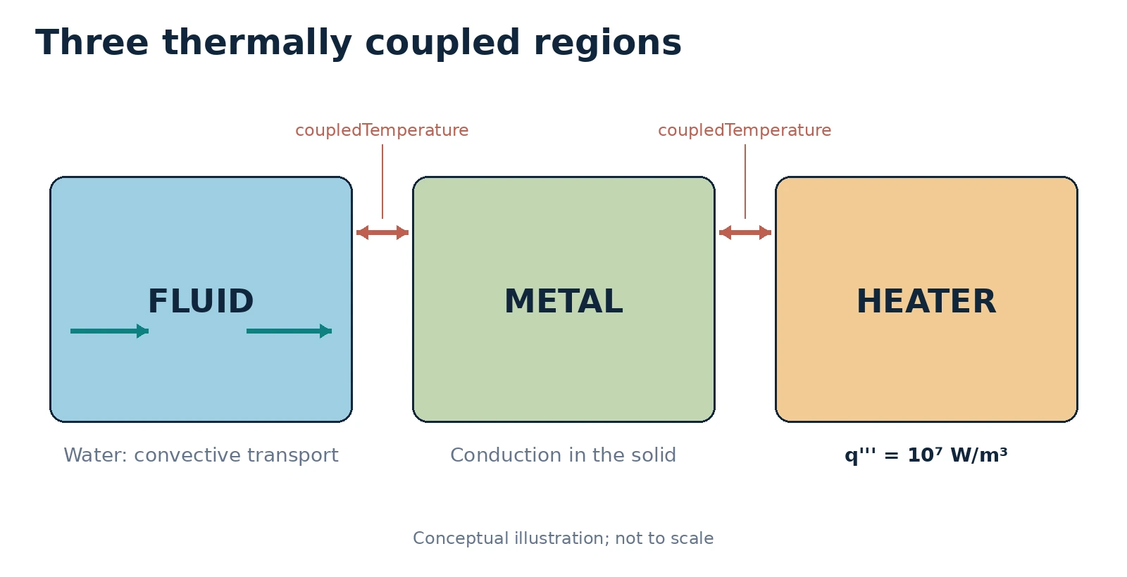
Three coupled regions: flowing fluid, conductive metal and heated solid
Environment: OpenFOAM Foundation 14 on Linux; ParaView 5.13.2, FileZilla and Notepad++ on Windows.
Level: intermediate · OpenFOAM series, guide 11 of 20
Aim. Prepare and run a CHT case in which fluid flows through a duct, a heater generates energy and a solid metal region conducts heat into the fluid. Change two parameters, inspect temperature fields, and evaluate the energy balance without confusing temperatures, total heat rates and heat flux densities.
1. Why conjugate heat transfer matters
Guides 1–10 covered remote operation, simulation logs, ParaView, numerical verification, automation, meshing, boundary conditions, transient flow, turbulence and natural convection. We now couple different physical media: the moving fluid transports thermal energy by advection and diffusion, while the stationary solid stores and conducts heat. Interface temperatures are calculated rather than arbitrarily prescribed.
For an ideal interface without contact resistance or surface sources, the temperature is continuous and normal heat flux is conserved; the outward fluxes of two adjoining regions have opposite signs. An apparent interface imbalance may reveal numerical, mesh-mapping or sign-convention problems. Do not conceal it by modifying the results after the calculation.
Optional refresher — units: temperature T [K]; conductivity k [W/(m K)]; surface heat flux q″ [W/m²]; heat-transfer rate Q̇ [W]; volumetric heat source q‴ [W/m³]. A surface flux and a volumetric source are not the same quantity.
Deep dive · Actual geometry of the case, read from the STL files
The three files in constant/geometry (heatedDuct.stl, fluidToMetal.stl, metalToHeater.stl) describe a simple geometry, with the duct axis along z:
| Region | Extent (mm) | Nominal volume | Notes |
|---|---|---|---|
fluid | x 5–45, y 5–45, z 0–150 | 2.40·10⁻⁴ m³ | square channel 40 × 40 mm, inlet 1.6·10⁻³ m² |
metal | x 0–50, y 0–50 minus the channel | 1.35·10⁻⁴ m³ | 5 mm wall on four sides |
heater | x 7.5–42.5, y −10–0, z 0–150 | 5.25·10⁻⁵ m³ | 35 × 10 mm plate under the duct |
The fluid-metal interface is the inner perimeter of the channel (4 × 40 mm × 150 mm = 0.024 m²); the metal-heater interface is the top face of the heater (35 × 150 mm = 5.25·10⁻³ m²). The heat generated in the heater must therefore first cross a small section and then spread along the metal wall: “circumferential” conduction in the metal is the physical key of the case. With the tutorial source the nominal power is Q̇gen = 10⁷ × 5.25·10⁻⁵ = 525 W; the actual value depends on the volume measured on the mesh (section 7).
Deep dive · Interface conditions and their discretisation
For an ideal interface between fluid (f) and solid (s), with normal n pointing out of the fluid:
T_f = T_s                                temperature continuity
kappa_f dT_f/dn = kappa_s dT_s/dn        normal flux continuity
In a finite-volume discretisation with the two adjacent cells at distances δf and δs from the face, these two conditions give an interface temperature weighted by the conductances:
T_i = (kappa_f/delta_f * T_f + kappa_s/delta_s * T_s) / (kappa_f/delta_f + kappa_s/delta_s)
q   = (T_s - T_f) / (delta_f/kappa_f + delta_s/kappa_s)
This is Patankar’s “harmonic mean” of conductivities: the flux is limited by the larger resistance. With water (κ = 0.61) and aluminium (κ = 200) and equal cells, the interface temperature is practically that of the metal: the resistance is all on the fluid side. This is why mesh quality on the fluid side decides the accuracy of the exchanged flux.
Practical tip · Dimensions in the files of this tutorial
Unlike Guide 10, the heatedDuct fields declare dimensions as a vector of seven exponents [mass length time temperature amount current luminous intensity]:
| Field | dimensions | SI |
|---|---|---|
0/*/T | [ 0 0 0 1 0 0 0 ] | K |
0/fluid/U | [ 0 1 -1 0 0 0 0 ] | m/s |
0/fluid/p, p_rgh | [ 1 -1 -2 0 0 0 0 ] | Pa |
A source in W/m³ has dimensions [1 −1 −3 0 0 0 0], a power in W [1 2 −3 0 0 0 0]: comparing the exponents is the quickest way to notice that q‴ and Q̇ have been swapped.
2. Verified Foundation 14 tutorial
This guide starts with the official $FOAM_TUTORIALS/multiRegion/CHT/heatedDuct case in the OpenFOAM Foundation 14 repository. It has three regions: fluid (water), metal (a heat-conducting solid) and heater (a solid containing a volumetric heat source). The regionSolvers dictionary in system/controlDict maps the regions onto fluid and solid modules. The appropriate executable is foamMultiRun. Do not blindly substitute legacy chtMultiRegionFoam commands from another OpenFOAM distribution.
| Region | Main fields | Physics | Files to inspect |
|---|---|---|---|
fluid | U, p, T | Flow and energy transport | 0/fluid/T, 0/fluid/U, constant/fluid/physicalProperties |
metal | T | Conduction in solid | 0/metal/T, constant/metal/physicalProperties |
heater | T | Conduction and source | 0/heater/T, constant/heater/fvModels |
The upstream tutorial specifies an inlet temperature of 300 K, prescribed velocity 0.001 m/s, reference metal conductivity 200 W/(m K) and volumetric heat generation 10⁷ W/m³. These are tutorial parameters, not experimental validation or a complete heat-exchanger design.
Deep dive · The tutorial data, file by file
| File | Content | Consequence |
|---|---|---|
system/controlDict | regionSolvers { fluid fluid; metal solid; heater solid; } | one module per region |
system/controlDict | endTime 20; deltaT 1e-3; adjustTimeStep yes; maxCo 1.0; writeInterval 1; writeFormat binary | 20 s of transient, writes every second in binary |
constant/fluid/momentumTransport | simulationType laminar; | no turbulence model |
constant/fluid/g | value (0 0 0); | zero gravity: no natural convection |
constant/fluid/physicalProperties | rhoConst, hConst, comment «Water» | constant density 1000 kg/m³ |
constant/metal/physicalProperties | comment “Aluminium”: ρ 2700, Cv 900, κ 200 | heSolidThermo, eConst |
constant/heater/physicalProperties | comment “Iron”: ρ 8000, Cv 450, κ 80 | heSolidThermo, eConst |
0/fluid/U | uniform inlet (0 0 1e-3) | undeveloped profile at the inlet |
0/fluid/T | inlet 300 K, outlet inletOutlet | handles possible backflow |
0/metal/T, 0/heater/T | zeroGradient on external faces | system adiabatic towards the outside |
The comments in the tutorial files associate the metal with aluminium and the heater with iron; properties are constant and rounded. The guide’s caution remains valid: changing only κ does not yield another real material (box in section 5).
Deep dive · Dimensionless numbers and time scales: what happens in 20 seconds
| Quantity | Value | Meaning |
|---|---|---|
| Re = U Dh/ν | 42 | laminar, consistent with the model |
| Pr | 6.62 | water at room temperature |
| Pe = Re Pr | 276 | axial transport dominated by convection |
| flow-through time L/U | 150 s | 7.5 times the simulated time |
| hydrodynamic entry length ≈ 0.05 Re Dh | 0.083 m | half the duct |
| thermal entry length ≈ 0.05 Re Pr Dh | 0.55 m | 3.7 times the duct: always developing |
| thermal penetration in water after 20 s √(αt) | 1.7 mm | the heated layer is thin |
| overall time constant Ctot/(ṁ cp) | ≈ 227 s | order of the time to approach steady state |
The consequence is clear: at t = 20 s the water entering from the inlet has travelled only 20 mm, and the water leaving is water present in the duct from the start, heated only near the walls. The outlet mixed-mean temperature is therefore still very close to 300 K and almost all the generated power is stored in the solids and in the water near the walls. The tutorial case is an initial transient, not a steady state: the balance of section 10 must include storage, exactly as the guide recommends.
Deep dive · Why gravity is zero and what would change
With g = (0 0 0) and constant density the flow does not depend on temperature: the thermal problem is decoupled from the flow problem. In a real test with water heated from below at 1 mm/s the situation would be the opposite. With β ≈ 2.76·10⁻⁴ 1/K and a 10 K difference over 40 mm, Gr = gβΔT D³/ν² ≈ 1.9·10⁶ and the Richardson number Gr/Re² ≈ 1000: natural convection would largely dominate forced convection, with transverse convective cells. The tutorial is therefore a numerical CHT demonstrator, not a model of a real apparatus. Studying mixed convection requires a new copy with non-zero g, an equation of state that lets density vary, and a mesh suited to the convective cells.
Practical tip · Reading values without opening the editor
cd "$FOAM_TUTORIALS/multiRegion/CHT/heatedDuct"
foamDictionary system/controlDict -entry regionSolvers
foamDictionary system/controlDict -entry endTime
foamDictionary constant/metal/physicalProperties -entry mixture/transport/kappa
foamDictionary constant/heater/fvModels -entry energySource/q
foamDictionary constant/fluid/g -entry value
foamDictionary reads and prints an entry, with the path separated by “/”. Used without write options it changes nothing: it is the safest way to check tutorial and copy parameters before each run.
3. Multi-region case organisation
heatedDuct/
├── 0/
│   ├── fluid/        T, U, p, p_rgh
│   ├── metal/        T
│   └── heater/       T
├── constant/
│   ├── fluid/        physicalProperties, momentumTransport, g
│   ├── metal/        physicalProperties
│   ├── heater/       physicalProperties, fvModels
│   └── geometry/     snappyHexMesh geometry
└── system/
    ├── controlDict   regionSolvers and time controls
    ├── blockMeshDict
    ├── snappyHexMeshDict
    ├── fluid/        fvSchemes, fvSolution
    ├── metal/        fvSchemes, fvSolution
    └── heater/       fvSchemes, fvSolution
The mesh is first built as a single domain and later split into region meshes. Each region has its own temperature field and material properties. Mesh discretisation affects geometric areas and volumes; quantitative heat-flow measurements must use the actual discretised geometry, not an assumed nominal area.
The official preparation sequence is blockMesh, snappyHexMesh, splitMeshRegions -cellZones all -defaultRegion fluid. The solution can then be executed in serial mode with foamMultiRun. The original Allrun uses parallel execution and reconstruction; do not mix the parallel and serial procedures inside the same case directory.
Deep dive · How the three-region mesh is built
blockMesh: a single block 20 × 24 × 60 = 28,800 cubic cells of 2.5 mm containing the whole geometry (x 0–50, y −10–50, z 0–150 mm, with a 0.001 mm margin).snappyHexMesh: refines to level 1 (1.25 mm cells) near the external surfaces and the two interfaces, snaps the mesh to the STL surfaces, adds no layers (addLayers false). ThefluidToMetalandmetalToHeatersurfaces create the faceZones of the same name and, withmode insidePoint, the cellZonesmetalandheater; the pointinsidePoint (0.025 0.025 0.075)lies in the fluid.splitMeshRegions -cellZones all -defaultRegion fluid: separates a mesh for each cellZone, assigns the remaining cells to thefluidregion and creates the interface patches named<region>_to_<region>.
With 1.25 mm cells the 5 mm metal wall is described by about 4 cells across its thickness and the heater by about 8. That is fine for a first study; for interface flux measurements it is the resolution on the water side that needs checking (box in section 1).
Practical tip · Inspecting the interfaces after splitting
cd "$HOME/OpenFOAM/CHT_Guida11/reference"
grep -A8 "fluid_to_metal" constant/fluid/polyMesh/boundary
grep -A8 "metal_to_fluid" constant/metal/polyMesh/boundary
grep -A8 "metal_to_heater" constant/metal/polyMesh/boundary
grep -A8 "heater_to_metal" constant/heater/polyMesh/boundary
Each interface patch must be of a “mapped” type naming the neighbouring region and patch, and the number of faces (nFaces) of the two patches in a pair must be equal: the regions come from the same mesh and the faces coincide. Different numbers or a wrong neighbouring region explain discontinuous interface temperatures (section 12).
Deep dive · The parallel path of Allrun, in a separate copy
The official Allrun decomposes into 4 subdomains with method hierarchical; n (1 1 4);, i.e. it cuts the duct into four sections along z. To use it in a new copy, after meshing:
decomposePar -allRegions > guide11_logs/decomposePar.log 2>&1
mpirun -np 4 foamMultiRun -parallel > guide11_logs/solve_parallel.log 2>&1
reconstructPar -allRegions > guide11_logs/reconstructPar.log 2>&1
With 28,800 starting cells the case is small and the parallel gain is modest; it mainly serves to test the procedure before finer meshes. Do not launch the parallel path in the same copy where solve_case.sh was run: serial and reconstructed results would end up in the same time folders.
4. What the physical modules solve
For an isotropic solid with constant properties, a simplified energy balance is:
ρₛ cₛ ∂T/∂t = ∇·(kₛ ∇T) + q‴
Within the fluid, energy also travels with the velocity field. The exact equation is governed by the thermophysical and turbulence models. Therefore the solution is more than two independent heat-diffusion calculations.
At adjoining region faces heat passes through the interface according to calculated temperature gradients. The coupledTemperature boundary condition appears on both sides of each coupled interface. In the official case the pairs are fluid_to_metal ↔ metal_to_fluid and metal_to_heater ↔ heater_to_metal.
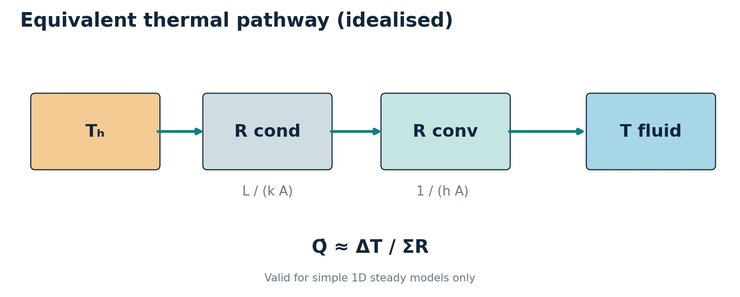
Optional refresher — resistances: for a simple one-dimensional idealisation, R_cond = L/(k A), R_conv = 1/(h A) and Q̇ ≈ ΔT/(R_cond + R_conv). These equations provide physical intuition but do not replace three-dimensional CHT calculations with nonuniform flow and geometry.
Deep dive · The equations assembled by the two modules
In the version 14 source the solid module (applications/modules/solid/solid.C) solves the sensible internal energy e for each solid region:
fvm::ddt(rho, e) + thermophysicalTransport->divq(e) == fvModels().source(rho, e)With eConst and rhoConst this is exactly ρ Cv ∂T/∂t = ∇·(κ∇T) + q‴, where q‴ comes from the heatSource in fvModels. The fluid module solves the sensible enthalpy h with convection, kinetic energy and pressure work (Guide 10); with g = 0 the buoyancy term is absent. The two families of equations are coupled only through the coupledTemperature conditions on the interface patches.
Deep dive · Time step, segregated coupling and accuracy in the solids
foamMultiRun solves the regions one after the other in a common outer PIMPLE loop. The time step is chosen as the minimum of the modules’ maxDeltaT: the fluid limits it with maxCo 1, while the version 14 solid module has no diffusion-number limit and only uses maxDeltaT from controlDict, if present. With U = 1 mm/s and 1.25 mm cells, the Courant number allows steps up to about 1 s. The cell Fourier number in aluminium then becomes Fo = αΔt/Δx² ≈ 8.2·10⁻⁵ × 1/(1.25·10⁻³)² ≈ 50.
The implicit Euler scheme remains stable, but with Fo ≫ 1 the time history in the solids is inaccurate, and with a single outer-loop pass the coupling between regions lags by one step. For a transient that you want to measure (section 10), in a new copy limit the step and increase the outer correctors:
// system/controlDict
maxDeltaT       0.05;

// system/fvSolution (top level, not system/<region>/fvSolution)
PIMPLE
{
    nOuterCorrectors 3;
}
The top-level PIMPLE block is the one that is empty in the tutorial; the official version 14 CHT tutorials set nOuterCorrectors there. The check is always the same: halve maxDeltaT and verify that the heater Tmax and stored energy do not change beyond the chosen tolerance.
Deep dive · Resistance network and fins: a prediction for exercise B
| Resistance | Estimate | Value |
|---|---|---|
| conduction across the metal thickness | 0.005 / (200 × 0.024) | 1.0·10⁻³ K/W |
| same, κ = 50 | 0.005 / (50 × 0.024) | 4.2·10⁻³ K/W |
| half heater thickness | 0.005 / (80 × 5.25·10⁻³) | 1.2·10⁻² K/W |
| water-side convection (h ≈ 350 W/(m² K)) | 1 / (350 × 0.024) | 0.12 K/W |
The h value is an order-of-magnitude estimate (κwater divided by the penetration thickness of about 1.7 mm). The convective resistance dominates: reducing the metal κ from 200 to 50 changes the series resistance little. It does, however, change the distribution a lot: the side and top walls act as fins fed from below. With the fin parameter m = √(h/(κ t)) and t = 5 mm, the side wall (45 mm) has efficiency ≈ 0.82 with κ = 200 and ≈ 0.55 with κ = 50 (cht_estimates.py). Hypothesis to test: with the less conductive metal the bottom wall and the heater become hotter, the side and top walls colder, and the power transferred to the water concentrates on the channel floor.
Deep dive · Additional script: cht_estimates.py
Collects all the estimates of this guide in one program: volumes and heat capacities, power, mass flow, Re, Pr, Pe, characteristic times, entry lengths, diffusion times, fin efficiency and hypothetical Richardson number. Nominal volumes should be replaced by the measured ones (--V-heater):
python cht_estimates.py
python cht_estimates.py --kappa-metal 50
python cht_estimates.py --q 5e6 --V-heater 5.31e-5
#!/usr/bin/env python3
# SPDX-License-Identifier: GPL-3.0-or-later
"""Hand estimates for the OpenFOAM 14 multiRegion/CHT/heatedDuct case.
Nominal geometry from the tutorial STL files: square duct 50 x 50 mm outside,
40 x 40 mm fluid channel (5 mm metal wall), heater 35 x 10 mm under the duct,
all 150 mm long. Properties from constant/*/physicalProperties. The numbers are
order-of-magnitude checks for the CFD results, not results themselves; the
volumes must be replaced by the values measured on the actual mesh
(checkMesh -region <name>, 'Total volume').
"""
import argparse
import math
def main():
p = argparse.ArgumentParser(description=__doc__)
p.add_argument('--q', type=float, default=1e7, help='heater source density [W/m3]')
p.add_argument('--kappa-metal', type=float, default=200.0, help='metal conductivity [W/(m K)]')
p.add_argument('--U', type=float, default=1e-3, help='inlet velocity [m/s]')
p.add_argument('--V-heater', type=float, help='measured heater volume [m3] (default: nominal)')
p.add_argument('--h', type=float, default=350.0, help='assumed fluid-side film coefficient [W/(m2 K)] for the fin estimate')
p.add_argument('--endTime', type=float, default=20.0, help='simulated time [s]')
a = p.parse_args()
L = 0.150
fluid = dict(rho=1000.0, c=4181.0, mu=959e-6, Pr=6.62, V=0.040 * 0.040 * L)
fluid['k'] = fluid['mu'] * fluid['c'] / fluid['Pr']
metal = dict(rho=2700.0, c=900.0, k=a.kappa_metal, V=(0.050 ** 2 - 0.040 ** 2) * L)
heater = dict(rho=8000.0, c=450.0, k=80.0, V=a.V_heater or 0.035 * 0.010 * L)
area_in = 0.040 * 0.040
dh = 0.040
nu = fluid['mu'] / fluid['rho']
mdot = fluid['rho'] * a.U * area_in
q_gen = a.q * heater['V']
re = a.U * dh / nu
pe = re * fluid['Pr']
print('Region V [m3] rho*c*V [J/K] alpha [m2/s] effusivity [W s^0.5/(m2 K)]')
total_c = 0.0
for name, r in (('fluid', fluid), ('metal', metal), ('heater', heater)):
cap = r['rho'] * r['c'] * r['V']
total_c += cap
alpha = r['k'] / (r['rho'] * r['c'])
eff = math.sqrt(r['k'] * r['rho'] * r['c'])
r['alpha'] = alpha
print(f'{name:7s} {r["V"]:.4e} {cap:12.1f} {alpha:.3e} {eff:9.0f}')
print(f'Water conductivity k = mu cp / Pr = {fluid["k"]:.4f} W/(m K)')
print(f'Heater power Q_gen = q * V_heater = {q_gen:.1f} W')
print(f'Mass flow rate = rho U A = {mdot:.4e} kg/s')
print(f'Re (D_h = 40 mm) = {re:.1f}, Pr = {fluid["Pr"]}, Pe = {pe:.0f}')
print(f'Flow-through time L/U = {L / a.U:.0f} s (simulated time {a.endTime:g} s)')
print(f'Hydrodynamic entry length ~ 0.05 Re D_h = {0.05 * re * dh:.3f} m')
print(f'Thermal entry length ~ 0.05 Re Pr D_h = {0.05 * pe * dh:.3f} m (duct length {L} m)')
print(f'Steady bulk temperature rise Q_gen/(mdot cp) = {q_gen / (mdot * fluid["c"]):.1f} K')
print(f'Lumped time constant C_total/(mdot cp) = {total_c / (mdot * fluid["c"]):.0f} s')
print(f'Energy generated up to endTime = {q_gen * a.endTime:.0f} J')
print(f'Adiabatic heater heating rate q/(rho c) = {a.q / (heater["rho"] * heater["c"]):.2f} K/s')
for name, r, d in (('metal wall (5 mm)', metal, 0.005), ('heater (10 mm)', heater, 0.010), ('water (5 mm)', fluid, 0.005)):
print(f'Diffusion time d^2/alpha, {name}: {d * d / r["alpha"]:.2f} s')
print(f'Thermal penetration in water after endTime sqrt(alpha t) = {1000 * math.sqrt(fluid["alpha"] * a.endTime):.2f} mm')
m = math.sqrt(a.h / (metal['k'] * 0.005))
for label, length in (('side wall (45 mm)', 0.045), ('side + top half (70 mm)', 0.070)):
ml = m * length
print(f'Fin estimate, {label}: mL = {ml:.2f}, efficiency tanh(mL)/mL = {math.tanh(ml) / ml:.2f}')
beta, dT, g = 2.76e-4, 10.0, 9.81
gr = g * beta * dT * dh ** 3 / nu ** 2
print(f'If gravity were active (beta = {beta} 1/K, dT = {dT} K): Gr = {gr:.2e}, Ri = Gr/Re^2 = {gr / re ** 2:.0f}')
if __name__ == '__main__':
main()Output for the reference case (excerpt):
Region   V [m3]      rho*c*V [J/K]   alpha [m2/s]   effusivity [W s^0.5/(m2 K)]
fluid    2.4000e-04        1003.4    1.449e-07           1591
metal    1.3500e-04         328.1    8.230e-05          22045
heater   5.2500e-05         189.0    2.222e-05          16971
Heater power Q_gen = q * V_heater = 525.0 W
Mass flow rate = rho U A = 1.6000e-03 kg/s
Flow-through time L/U = 150 s  (simulated time 20 s)
Steady bulk temperature rise Q_gen/(mdot cp) = 78.5 K
Lumped time constant C_total/(mdot cp) = 227 s
Adiabatic heater heating rate q/(rho c) = 2.78 K/s
Diffusion time d^2/alpha, metal wall (5 mm): 0.30 s
Diffusion time d^2/alpha, heater (10 mm): 4.50 s
Diffusion time d^2/alpha, water (5 mm): 172.58 s
5. Understand thermophysical properties before editing
The tutorial constant/fluid/physicalProperties represents water using 1000 kg/m³ reference density, Cp = 4181 J/(kg K), dynamic viscosity mu = 959e-6 Pa s, and Pr = 6.62. Metal conductivity is set to kappa = 200 W/(m K) and heater conductivity to 80 W/(m K). The supplied physical models use simple constant properties rather than temperature-dependent correlations.
In our first comparison, keep density, heat capacity and geometry unchanged. Change only kappa in constant/metal/physicalProperties from 200 to 50 W/(m K), and call it a hypothetical lower-conductivity solid. Do not claim that this represents a specific alternative metal unless density, capacity and other properties are made consistent.
The heat source is declared in constant/heater/fvModels:
energySource
{
    type       heatSource;
    cellZone   all;
    q          1e7;
}
Here q is a volumetric power density (W/m³), not the overall heater power. If the source acts throughout the heater region and is spatially uniform, the total rate is Q̇_gen = q‴ · V_heater, using the region volume measured on the actual mesh.
Deep dive · thermoType of the solids and of the fluid
| Entry | Fluid | Metal and heater |
|---|---|---|
type | heRhoThermo | heSolidThermo |
transport | const (μ, Pr → κ = μ cp/Pr) | constIsoSolid (constant isotropic κ) |
thermo | hConst (cp) | eConst (Cv) |
equationOfState | rhoConst | rhoConst |
energy | sensibleEnthalpy | sensibleInternalEnergy |
For the solids heat capacity is read under Cv, not Cp: with constant density the two coincide. In the fluid the hConst enthalpy is cp(T − Tref) plus the p/ρ contribution of the rhoConst equation of state, with Tref = 298.15 K unless specified (source hConstThermo.C); the p/ρ term is negligible here because gauge pressures are tiny.
Deep dive · Diffusivity and effusivity: who imposes the contact temperature
| Material | κ [W/(m K)] | ρc [J/(m³ K)] | α [m²/s] | e = √(κρc) |
|---|---|---|---|---|
| water | 0.606 | 4.18·10⁶ | 1.45·10⁻⁷ | 1 591 |
| metal (κ = 200) | 200 | 2.43·10⁶ | 8.23·10⁻⁵ | 22 045 |
| metal (κ = 50) | 50 | 2.43·10⁶ | 2.06·10⁻⁵ | 11 023 |
| heater | 80 | 3.60·10⁶ | 2.22·10⁻⁵ | 16 971 |
When two bodies at different temperatures are put in contact, the interface temperature is the average of the two weighted by the effusivities. The metal has an effusivity about 14 times that of water: in transients it imposes its own temperature on the interface and the water adapts. Diffusivity instead tells how fast heat spreads inside: in aluminium 570 times faster than in water, which is why the wall equalises within fractions of a second while the water stays cold a few millimetres from the wall.
Deep dive · heatSource: q per unit volume or total Q
In the version 14 source the heatSource model (src/fvModels/general/heatSource) requires either the total power Q [W] or the power density q [W/m³], both functions of time, applied to the given cellZone (all means all cells of the region). With q the actual power depends on the mesh volume; with Q it is fixed regardless of the mesh. In a mesh study a copy with the following is therefore convenient:
energySource
{
    type            heatSource;
    cellZone        all;
    Q               525;
}
so that differences between meshes do not include a change in the injected power. Only one of the two entries must be written: with both the model cannot know which to use.
Practical tip · A consistent alternative material
If a real, less conductive metal is of interest, change all properties together. For a carbon steel typical handbook values are κ ≈ 45–50 W/(m K), ρ ≈ 7850 kg/m³, c ≈ 460–490 J/(kg K). In a new copy:
// constant/metal/physicalProperties (mixture section)
equationOfState { rho 7850; }
transport       { kappa 50; }
thermodynamics  { hf 0; Cv 470; }
The volumetric heat capacity rises from 2.43·10⁶ to 3.69·10⁶ J/(m³ K): in the transient the metal heats more slowly for the same power. Comparing this case with lowConductivity separates the effect of conductivity from that of storage, which the “hypothetical” case mixes.
6. Prepare from Windows without overwriting existing work
Download the guide exercise bundle and transfer it to the server with FileZilla/SFTP, or run the scripts locally on the Linux server. Scripts require python3, bash and sourced OpenFOAM commands; Notepad++ is sufficient for Windows-side editing. Save shell files using Unix LF line endings.
ssh username@linux-server
source /opt/OpenFOAM-14/etc/bashrc    # adapt to local installation
foamVersion
python3 prepare_cases.py --output "$HOME/OpenFOAM/CHT_Guide11"
The preparation tool makes three new independent directories without changing the installed tutorial: reference, lowConductivity and lowHeatSource. The second uses metal conductivity 50 W/(m K); the third uses heater-source density 5×10⁶ W/m³. If any destination already exists, preparation stops instead of overwriting it.
Start by completing and checking reference before attempting the variants.
Deep dive · Package script: prepare_cases.py
#!/usr/bin/env python3
# SPDX-License-Identifier: GPL-3.0-or-later
"""Create isolated CHT tutorial variants without changing existing work."""
import argparse
import os
from pathlib import Path
import re
import shutil
import sys

CASES = {
    "reference": None,
    "lowConductivity": ("constant/metal/physicalProperties", "kappa", "50"),
    "lowHeatSource": ("constant/heater/fvModels", "q", "5e6"),
}


def replace_dictionary_scalar(file_path: Path, key: str, value: str) -> None:
    text = file_path.read_text(encoding="utf-8")
    pattern = rf"(?m)^(\s*{re.escape(key)}\s+)([0-9eE.+-]+)(\s*;)"
    matches = list(re.finditer(pattern, text))
    if len(matches) != 1:
        raise ValueError(f"Expected exactly one {key} scalar entry in {file_path}, found {len(matches)}")
    updated = re.sub(pattern, lambda match: match.group(1) + value + match.group(3), text, count=1)
    file_path.write_text(updated, encoding="utf-8")


def main() -> int:
    parser = argparse.ArgumentParser(description=__doc__)
    parser.add_argument("--output", required=True, type=Path, help="Directory containing NEW case folders")
    parser.add_argument("--tutorial", type=Path, help="Optional explicit path to the official heatedDuct case")
    args = parser.parse_args()
    tutorials = os.environ.get("FOAM_TUTORIALS", "")
    tutorial = args.tutorial or (Path(tutorials) / "multiRegion/CHT/heatedDuct" if tutorials else None)
    if not tutorial or not tutorial.is_dir():
        parser.error("Official heatedDuct tutorial not found; source OpenFOAM and set FOAM_TUTORIALS or use --tutorial")
    expected = ["system/controlDict", "constant/metal/physicalProperties", "constant/heater/fvModels", "0/fluid/T"]
    if any(not (tutorial / name).is_file() for name in expected):
        parser.error("The template is not the expected OpenFOAM Foundation 14 heatedDuct case")
    out = args.output.expanduser().resolve()
    if any((out / case).exists() for case in CASES):
        parser.error("One or more destination case directories already exist; refusing to overwrite")
    out.mkdir(parents=True, exist_ok=True)
    created = []
    try:
        for name, change in CASES.items():
            destination = out / name
            shutil.copytree(tutorial, destination, symlinks=False)
            created.append(destination)
            if change:
                relative, key, value = change
                replace_dictionary_scalar(destination / relative, key, value)
            (destination / "GUIDE11_CASE.txt").write_text(
                "Guide 11 (OpenFOAM Foundation 14)\n"
                f"Case name: {name}\n"
                f"Official source: {tutorial.resolve()}\n"
                f"Modification: {change or 'none'}\n"
                "Generated from a copy; upstream tutorial was not modified.\n",
                encoding="utf-8",
            )
            print(f"Prepared {destination}")
    except Exception as exc:
        # Preserve all created data to support forensic review; never clean up silently.
        print(f"Preparation stopped: {exc}. Existing copies were left in place.", file=sys.stderr)
        return 1
    return 0


if __name__ == "__main__":
sys.exit(main())replace_dictionary_scalarlooks for a line starting with the key (kappaorq) followed by a number and “;” and requires exactly one; otherwise it stops. In the official fileskappa 200;andq 1e7;appear only once.- Each copy receives a
GUIDE11_CASE.txtfile with origin and change: the mesh and solve scripts require it, so they cannot be launched by mistake on the installed tutorial. - If any of the three destinations exists, nothing is created. If an error occurs halfway, the copies already created are kept for analysis: the script never deletes.
- Run on the files of the official OpenFOAM 14 repository,
diff -r reference lowConductivityshows onlykappa 200;→kappa 50;and the description file;diff -r reference lowHeatSourceonlyq 1e7;→q 5e6;. A second run with the same destination ends with exit code 2.
Practical tip · Installation path and environment set-up
The command source /opt/OpenFOAM-14/etc/bashrc must be adapted: with the Ubuntu packages distributed by openfoam.org the typical path is /opt/openfoam14/etc/bashrc (lower case, no hyphen); with a source build it is in the user’s folder. To find and check it:
ls -d /opt/openfoam* /opt/OpenFOAM* 2>/dev/null
source /opt/openfoam14/etc/bashrc     # adjust to what ls shows
foamVersion
echo "$FOAM_TUTORIALS"
ls "$FOAM_TUTORIALS/multiRegion/CHT/heatedDuct"
The preparation script must be launched with its path (python3 scripts/prepare_cases.py from the package folder, as in the README) or after entering the scripts folder, as in the guide’s command.
Practical tip · Line endings and syntax check
cd ~/guide11_kit
file scripts/*.sh          # must NOT report "with CRLF line terminators"
bash -n scripts/mesh_case.sh && bash -n scripts/solve_case.sh && echo "syntax OK"
python3 -m py_compile scripts/prepare_cases.py scripts/energy_balance.py && echo "python OK"
If file reports CRLF, in Notepad++ use Edit → EOL Conversion → Unix (LF), save and transfer again with FileZilla in binary mode. bash -n checks syntax without running anything. py_compile creates a __pycache__ folder next to the scripts: it is harmless.
7. Meshing and pre-flight checks
cd "$HOME/OpenFOAM/CHT_Guide11/reference"
bash /path/to/scripts/mesh_case.sh "$PWD"
The script runs blockMesh, snappyHexMesh, splitMeshRegions -cellZones all -defaultRegion fluid, followed by regional checkMesh for fluid, metal and heater. Logs are stored under guide11_logs/; existing logs are never overwritten. The upstream tutorial is unchanged.
Confirm that all three constant/<region>/polyMesh directories exist and that the coupled patches are present. Review cell quality, non-orthogonality, and region interfaces. A successful checkMesh alone does not prove correct contact pairing. Use ParaView to inspect the three regions and geometry.
Deep dive · Package script: mesh_case.sh
#!/usr/bin/env bash
# SPDX-License-Identifier: GPL-3.0-or-later
# Mesh a fresh OpenFOAM Foundation 14 heatedDuct case and retain all logs.
set -euo pipefail
if [[ $# -ne 1 ]]; then
    echo "Usage: bash mesh_case.sh /absolute/path/to/case" >&2
    exit 2
fi
case_dir="$(realpath -- "$1")"
[[ -f "$case_dir/GUIDE11_CASE.txt" ]] || { echo "Not a prepared Guide 11 case: $case_dir" >&2; exit 2; }
command -v blockMesh >/dev/null || { echo "Source the OpenFOAM 14 environment first" >&2; exit 2; }
command -v snappyHexMesh >/dev/null || exit 2
command -v splitMeshRegions >/dev/null || exit 2
command -v checkMesh >/dev/null || exit 2
cd "$case_dir"
if [[ -d constant/fluid/polyMesh || -d constant/metal/polyMesh || -d constant/heater/polyMesh ]]; then
    echo "Regional meshes already exist; refusing to rebuild the case in place" >&2
    exit 1
fi
mkdir -p guide11_logs
run_logged() {
    local output="$1"; shift
    if [[ -e "$output" ]]; then
        echo "Existing log $output; refusing to overwrite" >&2
        return 1
    fi
    printf 'Running:'; printf ' %q' "$@"; printf '\n'
    "$@" > >(tee "$output") 2> >(tee -a "$output" >&2)
}
run_logged guide11_logs/mesh_blockMesh.log blockMesh
run_logged guide11_logs/mesh_snappyHexMesh.log snappyHexMesh
run_logged guide11_logs/mesh_splitMeshRegions.log splitMeshRegions -cellZones all -defaultRegion fluid
for region in fluid metal heater; do
    if [[ ! -f "constant/$region/polyMesh/boundary" ]]; then
        echo "No region mesh boundary file for $region" >&2
        exit 1
    fi
    run_logged "guide11_logs/checkMesh_${region}.log" checkMesh -region "$region"
done
printf 'Regional meshes created and checked in %s\n' "$case_dir"- The check on
GUIDE11_CASE.txtensures the case is a prepared copy; the check on the threepolyMeshfolders prevents re-meshing over an existing one. run_loggedprints the command, writes the output to screen and to the log withtee(errors too, withtee -a) and refuses to reuse an existing log.- After
splitMeshRegionsit checks thatconstant/<region>/polyMesh/boundaryexists for each region before launchingcheckMesh -region.
Practical tip · Heater volume and actual power
cd "$HOME/OpenFOAM/CHT_Guida11/reference"
grep -E "cells:|Total volume" guide11_logs/checkMesh_fluid.log guide11_logs/checkMesh_metal.log guide11_logs/checkMesh_heater.log
checkMesh prints the cell count and, in the geometry check, the total volume of the region. Expected for the heater: about 5.25·10⁻⁵ m³. The actual power is Q̇gen = 10⁷ × Vheater: a 2 % difference in volume is a 2 % difference in power, to be used in the balance instead of the nominal 525 W. Also record the volumes of fluid and metal: they are needed for the heat capacities of section 10.
Practical tip · What to look at in checkMesh for each region
- “Mesh OK” at the end of each of the three logs; otherwise read which checks fail.
- Maximum non-orthogonality: the cells cut by
snappyHexMeshnear the interfaces are the most distorted; beyond about 70° non-orthogonal correctors are needed. - Patch list: in the fluid
fluidInlet,fluidOutlet,fluid_to_metal; in the metalmetalInlet,metalOutlet,metalExternal,metal_to_fluid,metal_to_heater; in the heaterheaterInlet,heaterOutlet,heaterExternal,heater_to_metal. - Inlet, outlet or interface patches with zero faces, or regions with different cell counts across the three prepared copies (which use the same geometry and meshing dictionary): they indicate a mesh problem, not a physics one.
8. Run the coupled solution and inspect logs
bash /path/to/scripts/solve_case.sh "$HOME/OpenFOAM/CHT_Guide11/reference"
tail -n 35 "$HOME/OpenFOAM/CHT_Guide11/reference/guide11_logs/solve_foamMultiRun.log"
The run script verifies that region meshes exist and refuses to overwrite an existing solver log. It does not silently restart a partially completed calculation. Use tmux for detached sessions, as described in Guide 1. Retrieve logs to Windows with FileZilla when needed.
Look for interface-coupling errors, unstable energy residuals, Courant numbers and solver runtime. Linear-solver residuals are not the same as a physical energy-conservation audit; perform that separately.
Deep dive · Package script: solve_case.sh
#!/usr/bin/env bash
# SPDX-License-Identifier: GPL-3.0-or-later
# Run a meshed CHT tutorial case once; do not silently restart old solutions.
set -euo pipefail
if [[ $# -ne 1 ]]; then
    echo "Usage: bash solve_case.sh /absolute/path/to/case" >&2
    exit 2
fi
case_dir="$(realpath -- "$1")"
[[ -f "$case_dir/GUIDE11_CASE.txt" ]] || { echo "Not a prepared Guide 11 case" >&2; exit 2; }
command -v foamMultiRun >/dev/null || { echo "Source the OpenFOAM 14 environment first" >&2; exit 2; }
cd "$case_dir"
for region in fluid metal heater; do
    [[ -f "constant/$region/polyMesh/boundary" ]] || { echo "Missing $region mesh" >&2; exit 1; }
done
mkdir -p guide11_logs
log="guide11_logs/solve_foamMultiRun.log"
if [[ -e "$log" ]]; then
    echo "Solver log already exists; refusing to overwrite or restart" >&2
    exit 1
fi
# Use one serial solver process; the official Allrun is a separate MPI workflow.
foamMultiRun > >(tee "$log") 2> >(tee -a "$log" >&2)
printf 'Solver finished; log: %s/%s\n' "$case_dir" "$log"
The script checks the description file, the availability of foamMultiRun and the three region meshes, then runs the serial computation once, saving output and errors in guide11_logs/solve_foamMultiRun.log. The final comment recalls that the official Allrun is a separate MPI path.
Deep dive · Measuring during the run: a system/functions file for CHT
Balance quantities are best measured by OpenFOAM itself, at every step and on the actual mesh. In a prepared copy that already has its mesh, before solve_case.sh, save this file as system/functions (OpenFOAM 14 reads it automatically):
/*--------------------------------*- C++ -*----------------------------------*\
  Guide 11 - monitoring functions for a NEW copy of heatedDuct.
  Save as <case>/system/functions before running solve_case.sh.
\*---------------------------------------------------------------------------*/
FoamFile
{
    format      ascii;
    class       dictionary;
    location    "system";
    object      functions;
}

// Mass flow rate [kg/s]: in the fluid module phi is a mass flux.
#includeFunc patchFlowRate(name=mdotIn, region=fluid, patch=fluidInlet)
#includeFunc patchFlowRate(name=mdotOut, region=fluid, patch=fluidOutlet)

// Signed enthalpy flow sum(phi*h) [W]: negative on the inlet, positive on the outlet.
// Q_fluid = hFlowOut + hFlowIn
hFlowIn
{
    type            surfaceFieldValue;
    libs            ("libfieldFunctionObjects.so");
    writeControl    timeStep;
    writeInterval   1;
    log             yes;
    writeFields     false;
    region          fluid;
    patch           fluidInlet;
    operation       sum;
    weightField     phi;
    fields          (h);
}

hFlowOut
{
    type            surfaceFieldValue;
    libs            ("libfieldFunctionObjects.so");
    writeControl    timeStep;
    writeInterval   1;
    log             yes;
    writeFields     false;
    region          fluid;
    patch           fluidOutlet;
    operation       sum;
    weightField     phi;
    fields          (h);
}

// Mass-flow-weighted (bulk) temperatures [K]: sum(phi*T)/sum(phi).
TbulkIn
{
    type            surfaceFieldValue;
    libs            ("libfieldFunctionObjects.so");
    writeControl    timeStep;
    writeInterval   1;
    log             yes;
    writeFields     false;
    region          fluid;
    patch           fluidInlet;
    operation       average;
    weightField     phi;
    fields          (T);
}

TbulkOut
{
    type            surfaceFieldValue;
    libs            ("libfieldFunctionObjects.so");
    writeControl    timeStep;
    writeInterval   1;
    log             yes;
    writeFields     false;
    region          fluid;
    patch           fluidOutlet;
    operation       average;
    weightField     phi;
    fields          (T);
}

// Volume-averaged temperatures [K]: stored energy E = rho*c*V*Tavg + const.
#includeFunc volAverage(name=TavgFluid, region=fluid, T)
#includeFunc volAverage(name=TavgMetal, region=metal, T)
#includeFunc volAverage(name=TavgHeater, region=heater, T)

// Hottest cell of the heater [K].
#includeFunc cellMax(name=TmaxHeater, region=heater, T)

// Heat flow through every wall patch of each region [W], positive = into the region.
// Interface check: Q(fluid_to_metal) = -Q(metal_to_fluid), Q(metal_to_heater) = -Q(heater_to_metal).
#includeFunc wallHeatFlux(name=qFluid, region=fluid, writeFields=false, log=yes)
#includeFunc wallHeatFlux(name=qMetal, region=metal, writeFields=false, log=yes)
#includeFunc wallHeatFlux(name=qHeater, region=heater, writeFields=false, log=yes)

// ************************************************************************* //patchFlowRatesums the fluxphiover the patch: in thefluidmodule it is a mass flux, so the result is ṁ in kg/s (negative at the inlet).- With
operation sumandweightField phithesurfaceFieldValuecomputes Σ φf hf, the signed enthalpy flow. Q̇fluid = hFlowOut + hFlowIn is the net power carried away by the water, already corrected for any backflow. - With
operation averageandweightField phione obtains Σ φT/Σ φ: the flow-weighted mean temperature of section 9. wallHeatFluxper region gives the power on each wall patch, positive when entering the region: Q(fluid_to_metal) is the heat entering the water, and must equal −Q(metal_to_fluid).
Operations and weights are checked in the version 14 surfaceFieldValue source; the syntax follows the official tutorials wallBoiling, hotWire and vacuumFurnace. At start-up the log must list the creation of every function object and, at every step, the values. The files end up under postProcessing/: find postProcessing -name "*.dat" lists them all.
Practical tip · Reading a multi-region log
L="$HOME/OpenFOAM/CHT_Guida11/reference/guide11_logs/solve_foamMultiRun.log"
grep -c "^Time = " "$L"                    # steps performed
grep "^deltaT = " "$L" | tail -3            # current step
grep "Courant Number" "$L" | tail -3
grep "Solving for h" "$L" | tail -3        # fluid
grep "Solving for e" "$L" | tail -6        # metal and heater
grep -i -E "warning|error|nan" "$L" | head
The step must grow from 10⁻³ s up to the Courant limit and then settle. “Solving for e” appears twice per step, once for each solid region. The computing time per simulated second, read from ExecutionTime, allows the duration of a copy with a longer endTime to be estimated before launching it.
9. ParaView quantitative analysis from Windows
Connect ParaView 5.13.2 to the Linux pvserver as covered by Guide 1. Select each required region in the OpenFOAM reader, checking which time steps, volume meshes and boundary patches are exposed. When displayed together, the fluid, metal and heater have distinct temperature arrays even if each is called T.
A useful visual sequence is heater T → metal T → fluid T → fluid velocity. Create longitudinal and transverse Slice filters, use a common temperature range for comparisons, save the ParaView state .pvsm, and always record time, region, physical units and colour limits.
For convective energy transport use mass-flow rate and a mass-flow-weighted temperature, not a plain arithmetic average of face or node temperatures:
T̄_m = [∫ₐ T ρ (U·n) dA] / [∫ₐ ρ (U·n) dA]
The signed normal mass flux changes sign between inlet and outlet. Treat recirculating/backflow faces explicitly; a single average can be misleading in those circumstances.
Deep dive · ParaView with a multi-region case
- Create the empty opening file in the case folder:
touch reference.foam. Opening it from ParaView connected topvserver, the OpenFOAM reader shows the internal meshes and patches of each region in “Mesh Regions”, prefixed by the region name. - Select the three internal meshes and press Apply; with Extract Block separate the regions to colour them independently. The field is called
Tin all three: after extraction it is clear which region it belongs to. - The case is written in binary (
writeFormat binary): ParaView reads it without problems, but the files cannot be inspected with a text editor. - For a computation run in parallel and not reconstructed, set “Case Type” to Decomposed Case.
Practical tip · A profile through the three regions
With Plot Over Line from (0.025, −0.010, 0.075) to (0.025, 0.045, 0.075) you cross, at mid-length, the heater, the metal floor and the water. Flux continuity requires the slopes on either side of an interface to be in the inverse ratio of the conductivities: at the metal-water interface the gradient in the water must be about 330 times that in aluminium (200/0.606). In the plot the temperature looks almost flat in the metal and steep in the water: if the transition between the two regions is not continuous, the coupling is not working.
Deep dive · The mixed-mean temperature computed by OpenFOAM
The guide’s formula coincides with what the TbulkIn and TbulkOut function objects compute (section 8): on boundary faces φf = ρ (U·n) Af, and Σ φfTf/Σ φf is the discrete version of ∫ρT(U·n)dA/∫ρ(U·n)dA. For an already written time, without re-running, foamPostProcess can be used on the fluid region alone, with the explicit solver so that phi is available:
cd "$HOME/OpenFOAM/CHT_Guida11/reference"
foamPostProcess -region fluid -solver fluid -latestTime \
  -func "patchFlowRate(patch=fluidOutlet)" > guide11_logs/post_mdot_outlet.log 2>&1
grep -A3 "patchFlowRate" guide11_logs/post_mdot_outlet.log
The -solver option is also needed for wallHeatFlux (Guide 10): without it, foamPostProcess reads the fields but does not construct the thermal transport model. For the solid regions use -region metal -solver solid.
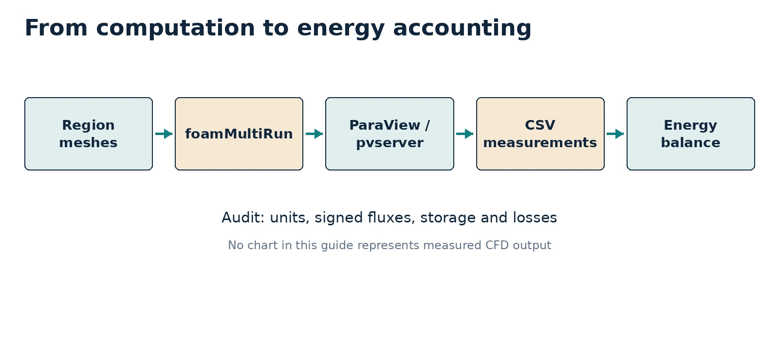
10. Energy accounting and quantitative comparison
Under approximately steady-state conditions with known mass flow and heat capacity, fluid heat uptake can be estimated as:
Q̇_fluid ≈ ṁ · cₚ · (T̄_out − T̄_in)
For an adiabatic, steady system with negligible storage, the expectation is Q̇_gen ≈ Q̇_fluid. At intermediate transient times the solid and fluid regions store energy, and any external heat losses must be included:
Q̇_gen − Q̇_fluid − Q̇_ext = dE_stored/dt
A transient discrepancy does not automatically indicate a solver problem: quantify storage and external fluxes before drawing conclusions. The supplied energy_balance.py reads a CSV with measured m_dot_kg_s, T_in_K, T_out_K, cp_J_kgK, q_gen_W, q_ext_W, dE_dt_W; it computes the signed balance residual. The sample CSV is illustrative only, never presented as OpenFOAM output.
Deep dive · What to expect from the balance at t = 20 s
| Term | Estimate | Comment |
|---|---|---|
| Q̇gen | ≈ 525 W | constant from the first step |
| energy generated in 20 s | ≈ 10.5 kJ | Q̇gen × 20 s |
| ṁ cp(T̄out − T̄in) | close to zero | heated water has not yet reached the outlet |
| dEstored/dt | almost all of Q̇gen | solids and water near the walls |
| heat across the water interface Q(fluid_to_metal) | growing fraction | enters the water but stays stored there |
Two often confused quantities must therefore be kept separate: the heat crossing the wall into the water (measured by wallHeatFlux) and the heat the water carries out of the domain (ṁ cpΔT). Their difference is the energy stored in the water. Only in steady state do they coincide, and then they equal Q̇gen.
Deep dive · Reaching steady state: times and a physical limit
Steady state requires a few overall time constants (≈ 227 s) plus the flow-through time (150 s): an endTime of 1500–2000 s in a new copy. Under those conditions the balance would give ΔT̄ = Q̇gen/(ṁ cp) = 525/(1.6·10⁻³ × 4181) ≈ 78.5 K, i.e. outlet water at about 378 K: beyond boiling at atmospheric pressure, with even hotter walls. The constant-density, single-phase model cannot represent that. For a physically sensible steady study reduce the power (for example q 1e6, ΔT̄ ≈ 7.9 K) or increase the inlet velocity, always in a new copy and documenting the choice.
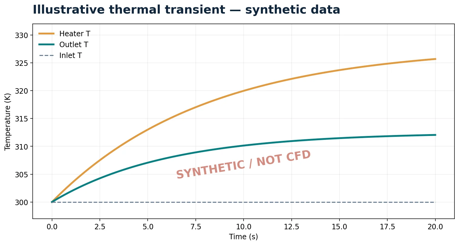
Note on the synthetic figure: the “fluid outlet” curve rises to 312 K in 20 s, while the estimates indicate an almost unchanged outlet mixed-mean temperature in that interval. The figure illustrates the shape of a transient, not a prediction for this case.
Deep dive · Package script: energy_balance.py
#!/usr/bin/env python3
# SPDX-License-Identifier: GPL-3.0-or-later
"""Evaluate signed CHT energy balance from measured CSV rows, not CFD files."""
import argparse
import csv
from pathlib import Path
import sys

REQUIRED = ["case", "time_s", "m_dot_kg_s", "T_in_K", "T_out_K", "cp_J_kgK", "q_gen_W", "q_ext_W", "dE_dt_W"]


def parse_float(row, key, number):
    try:
        value = float(row[key])
    except (ValueError, KeyError, TypeError) as exc:
        raise ValueError(f"Row {number}: invalid {key}") from exc
    if not -float("inf") < value < float("inf"):
        raise ValueError(f"Row {number}: {key} is not finite")
    return value


def main():
    parser = argparse.ArgumentParser(description=__doc__)
    parser.add_argument("input_csv", type=Path)
    parser.add_argument("--output", type=Path, help="New output CSV; existing files are never overwritten")
    args = parser.parse_args()
    target = args.output or args.input_csv.with_name(args.input_csv.stem + "_balance.csv")
    if target.resolve() == args.input_csv.resolve() or target.exists():
        parser.error("Output is the input or already exists: no overwriting")
    with args.input_csv.open(encoding="utf-8-sig", newline="") as source:
        reader = csv.DictReader(source)
        if not reader.fieldnames or any(key not in reader.fieldnames for key in REQUIRED):
            parser.error("Required columns: " + ", ".join(REQUIRED))
        entries = []
        for number, row in enumerate(reader, 2):
            data = {key: parse_float(row, key, number) for key in REQUIRED[1:]}
            q_fluid = data["m_dot_kg_s"] * data["cp_J_kgK"] * (data["T_out_K"] - data["T_in_K"])
            residual = data["q_gen_W"] - q_fluid - data["q_ext_W"] - data["dE_dt_W"]
            denom = max(abs(data["q_gen_W"]), 1e-12)
            entries.append(dict(row, q_fluid_W=f"{q_fluid:.12g}", residual_W=f"{residual:.12g}", residual_percent_source=f"{100*residual/denom:.9g}"))
    with target.open("x", encoding="utf-8", newline="") as out:
        writer = csv.DictWriter(out, fieldnames=reader.fieldnames + ["q_fluid_W", "residual_W", "residual_percent_source"])
        writer.writeheader()
        writer.writerows(entries)
    print(f"Wrote {len(entries)} rows to {target}")
    print("Convention: q_gen - q_fluid - q_ext - dE/dt = residual; positive q_ext is heat leaving the system.")
    print("This arithmetic does not prove that the CFD measurements are correct.")
    return 0


if __name__ == "__main__":
sys.exit(main())- Required columns:
case, time_s, m_dot_kg_s, T_in_K, T_out_K, cp_J_kgK, q_gen_W, q_ext_W, dE_dt_W. For each row it computes qfluid = ṁ cp(Tout − Tin) and the residual qgen − qfluid − qext − dE/dt, also as a percentage of the source. - Without
--outputit writes next to the input a file with suffix_balance.csv, refusing to overwrite it. - Convention printed at the end: positive qext is heat leaving the system.
- Run on the package synthetic CSV it produces a file identical to
example_measured_values_SYNTHETIC_balance.csv. The 0.02 W residual of thereferencerow comes from rounding of Tout in the example file, not from the computation.
Deep dive · Package exercise files
esercitazione/measurement_template.csv
case,time_s,m_dot_kg_s,T_in_K,T_out_K,cp_J_kgK,q_gen_W,q_ext_W,dE_dt_Wesercitazione/example_measured_values_SYNTHETIC.csv (invented values)
case,time_s,m_dot_kg_s,T_in_K,T_out_K,cp_J_kgK,q_gen_W,q_ext_W,dE_dt_W
reference,10,0.004,300,309.565893326,4181,1000,100,740
lowConductivity,10,0.004,300,305.979430758,4181,1000,100,800
lowHeatSource,10,0.004,300,305.979430758,4181,500,50,350
esercitazione/example_measured_values_SYNTHETIC_balance.csv (expected output)
case,time_s,m_dot_kg_s,T_in_K,T_out_K,cp_J_kgK,q_gen_W,q_ext_W,dE_dt_W,q_fluid_W,residual_W,residual_percent_source
reference,10,0.004,300,309.565893326,4181,1000,100,740,159.979999984,0.0200000159764,0.0020000016
lowConductivity,10,0.004,300,305.979430758,4181,1000,100,800,99.9999999968,3.20835624734e-09,3.20835625e-10
lowHeatSource,10,0.004,300,305.979430758,4181,500,50,350,99.9999999968,3.20835624734e-09,6.41671249e-10
esercitazione/README_IT_EN.md
# Guida 11 — Materiale di esercitazione / Exercise kit

**IT** — Questa cartella contiene tre strumenti: `prepare_cases.py` (copia il tutorial ufficiale e prepara tre casi indipendenti), `mesh_case.sh` (costruisce e controlla le mesh regionali) e `solve_case.sh` (esegue la soluzione seriale con `foamMultiRun`). `energy_balance.py` elabora esclusivamente misure registrate in un CSV; non legge automaticamente i campi OpenFOAM. I file sorgente e tutti i commenti nel codice sono in inglese. Gli script non sovrascrivono log, simulazioni o file di output già esistenti. Occorre avere OpenFOAM Foundation 14 attivato nel terminale Linux.

**EN** — This directory contains `prepare_cases.py` (copies the upstream tutorial and prepares three independent cases), `mesh_case.sh` (generates and checks the region meshes), and `solve_case.sh` (runs the serial solution using `foamMultiRun`). `energy_balance.py` processes values that **you measured and entered** into CSV; it does not automatically extract fields from OpenFOAM. The scripts do not overwrite prior cases, solver logs or outputs. Source OpenFOAM Foundation 14 in the Linux shell before running the scripts.

```bash
source /opt/OpenFOAM-14/etc/bashrc
python3 scripts/prepare_cases.py --output "$HOME/OpenFOAM/CHT_Guide11"
bash scripts/mesh_case.sh "$HOME/OpenFOAM/CHT_Guide11/reference"
bash scripts/solve_case.sh "$HOME/OpenFOAM/CHT_Guide11/reference"
python3 scripts/energy_balance.py esercitazione/example_measured_values_SYNTHETIC.csv
```

**Warning:** the output CSV generated by the last command is based on **synthetic test values**, not on a completed CFD simulation. The real heater power depends on the *actual* heater region volume and mesh. The transient energy balance must include internal energy storage and external losses where applicable. The included `measurement_template.csv` is intentionally empty and requires measured values.

**Official case:** https://github.com/OpenFOAM/OpenFOAM-14/tree/master/tutorials/multiRegion/CHT/heatedDuct
**Licence for new scripts:** GNU GPL v3 or later. The upstream OpenFOAM case is **not redistributed** in this bundle; it is copied from the user's installed OpenFOAM tutorial directory.
Deep dive · Additional script: cht_balance_series.py
Computes the transient balance step by step from the files of the section 8 function objects. With constant density and specific heats the energy of a region is E = ρcV·T̄vol + constant, so its derivative follows from the mean temperatures by central differences. The capacities C = ρcV are computed with the volumes measured by checkMesh:
cd "$HOME/OpenFOAM/CHT_Guida11/reference"
find postProcessing -name "*.dat"
# example with nominal volumes: fluid 1000*4181*2.4e-4, metal 2700*900*1.35e-4, heater 8000*450*5.25e-5
python3 cht_balance_series.py --qgen 525 \
  --hin  <path>/hFlowIn/.../surfaceFieldValue.dat \
  --hout <path>/hFlowOut/.../surfaceFieldValue.dat \
  --region fluid:<path>/TavgFluid/.../volFieldValue.dat:1003.4 \
  --region metal:<path>/TavgMetal/.../volFieldValue.dat:328.1 \
  --region heater:<path>/TavgHeater/.../volFieldValue.dat:189.0 \
  --every 20 --output ../reference_balance_series.csv
#!/usr/bin/env python3
# SPDX-License-Identifier: GPL-3.0-or-later
"""Transient energy balance of a CHT run from OpenFOAM function-object files.
Inputs are the .dat files written by the monitoring functions of Guide 11:
--hin / --hout surfaceFieldValue 'sum' of h weighted by phi on the fluid
inlet and outlet [W] (signed: negative on the inlet);
--region NAME:FILE:C volume-averaged temperature of a region and its
heat capacity C = rho*c*V [J/K] (V measured with checkMesh).
With constant density and specific heat the stored energy of a region is
E = C * T_avg + const, so dE/dt follows from finite differences in time.
Balance: residual = Q_gen - Q_fluid - Q_ext - dE/dt, Q_fluid = hout + hin.
The first column of each file is time, the selected column (default 2) the
value. A NEW output CSV is written; existing files are never overwritten.
"""
import argparse
import csv
from pathlib import Path
import sys
def read_series(path, column):
t, v = [], []
with open(path, encoding='utf-8') as f:
for number, line in enumerate(f, 1):
s = line.strip()
if not s or s.startswith('#'):
continue
parts = s.replace('(', ' ').replace(')', ' ').split()
try:
t.append(float(parts[0]))
v.append(float(parts[column - 1]))
except (IndexError, ValueError) as exc:
raise ValueError(f'{path}:{number}: cannot read column {column}') from exc
if len(t) < 3:
raise ValueError(f'{path}: at least three records are needed')
pairs = sorted(dict(zip(t, v)).items())
return [p[0] for p in pairs], [p[1] for p in pairs]
def interp(ts, vs, x):
if x <= ts[0]:
return vs[0]
if x >= ts[-1]:
return vs[-1]
lo, hi = 0, len(ts) - 1
while hi - lo > 1:
mid = (lo + hi) // 2
if ts[mid] <= x:
lo = mid
else:
hi = mid
w = (x - ts[lo]) / (ts[hi] - ts[lo])
return vs[lo] + w * (vs[hi] - vs[lo])
def main():
p = argparse.ArgumentParser(description=__doc__, formatter_class=argparse.RawDescriptionHelpFormatter)
p.add_argument('--qgen', type=float, required=True, help='heater power [W] = q * V_heater')
p.add_argument('--qext', type=float, default=0.0, help='heat leaving through external walls [W]')
p.add_argument('--hin', type=Path, required=True)
p.add_argument('--hout', type=Path, required=True)
p.add_argument('--region', action='append', required=True, help='NAME:FILE:C, repeat for each region')
p.add_argument('--column', type=int, default=2, help='value column in the .dat files')
p.add_argument('--every', type=int, default=1, help='keep one output row every N time records')
p.add_argument('--output', type=Path, required=True)
a = p.parse_args()
if a.output.exists():
p.error('Output already exists; refusing to overwrite it')
hin = read_series(a.hin, a.column)
hout = read_series(a.hout, a.column)
regions = []
for spec in a.region:
try:
name, file_name, cap = spec.rsplit(':', 2)
regions.append((name, read_series(Path(file_name), a.column), float(cap)))
except ValueError as exc:
p.error(f'bad --region {spec}: {exc}')
times = regions[0][1][0]
energy = [sum(c * interp(s[0], s[1], t) for _, s, c in regions) for t in times]
rows = []
for i in range(1, len(times) - 1, max(1, a.every)):
t = times[i]
dedt = (energy[i + 1] - energy[i - 1]) / (times[i + 1] - times[i - 1])
q_fluid = interp(*hout, t) + interp(*hin, t)
residual = a.qgen - q_fluid - a.qext - dedt
rows.append(dict(time_s=f'{t:.6g}', Q_gen_W=f'{a.qgen:.6g}', Q_fluid_W=f'{q_fluid:.6g}',
dE_dt_W=f'{dedt:.6g}', residual_W=f'{residual:.6g}',
residual_percent=f'{100 * residual / a.qgen:.4g}' if a.qgen else 'nan'))
with a.output.open('x', newline='', encoding='utf-8') as f:
w = csv.DictWriter(f, fieldnames=list(rows[0]))
w.writeheader()
w.writerows(rows)
last = rows[-1]
print(f'{len(rows)} rows written to {a.output}')
print(f"Last row t = {last['time_s']} s: Q_fluid = {last['Q_fluid_W']} W, dE/dt = {last['dE_dt_W']} W, "
f"residual = {last['residual_W']} W ({last['residual_percent']} % of Q_gen)")
print('Central differences need closely spaced records; check the residual for sensitivity to --every.')
if __name__ == '__main__':
try:
main()
except (OSError, ValueError) as exc:
sys.exit(f'ERROR: {exc}')Tested on analytic series built so that the terms sum to zero: the computed residual stays below 10⁻³ W out of 525 W. On real data a residual of a few percent in the first steps is normal (small steps, central differences on a fast transient); a residual that does not decrease with finer steps indicates a wrong measurement or a conservation problem at the interface, to be checked with the wallHeatFlux values of the two regions. Replace <path> with the paths listed by find.
11. Three practical exercises
A — Official reference. Create reference, mesh it, solve it, visualise the three regions, and record inlet/outlet temperatures, mass-flow rate and heater volume. Archive logs and ParaView state.
B — Solid conductivity. Compare reference with lowConductivity. Compare solid temperature profiles, fluid outlet mixed temperature and total transferred heat. State your hypothesis first: reduced conductivity does not guarantee monotonic changes in all local temperatures during transient conditions.
C — Heater power. Compare reference and lowHeatSource, reporting volumetric heat-source density, maximum temperature, energy storage and fluid outlet temperature. Do not assume linear scaling if other physics or properties change.
| Case | Metal k [W/(m K)] | Heater q‴ [W/m³] | Outlet T [K] | Fluid Q̇ [W] | Status |
|---|---|---|---|---|---|
| reference | 200 | 1.0×10⁷ | measure | measure | not run |
| lowConductivity | 50 | 1.0×10⁷ | measure | measure | not run |
| lowHeatSource | 200 | 5.0×10⁶ | measure | measure | not run |
Deep dive · Exercise C as a verification test: the problem is linear
In this tutorial all properties are constant, gravity is zero and density does not depend on T: the flow field is identical in the three cases and the energy equation is linear in the difference T − 300 K, with a source proportional to q‴. The time steps also coincide, because they depend only on velocity. An exact prediction follows: in lowHeatSource every temperature increase must be exactly half that of reference, in every cell and at every instant.
(T_lowHeatSource - 300) / (T_reference - 300) = 0.5The measured deviation, for example on the heater Tmax and on the mean temperatures from the function objects, directly gives the order of the linear-solver tolerance error. The guide rightly notes that temperatures do not scale linearly if the convective field or the properties change: here, by construction, they do not change, and the test exploits exactly that. If the deviation exceeds a few thousandths, check that the two copies really differ only in q (diff -r).
Practical tip · A more complete measurement sheet
| Case | Vheater [m³] | Q̇gen [W] | Tmax,heater [K] | T̄out [K] | Q(fluid_to_metal) [W] | ṁcpΔT [W] | dE/dt [W] | residual [%] |
|---|---|---|---|---|---|---|---|---|
| reference | … | … | … | … | … | … | … | … |
| lowConductivity | … | … | … | … | … | … | … | … |
| lowHeatSource | … | … | … | … | … | … | … | … |
Fill one row per case at the same instant (t = 20 s) and always state: instant, tolerances, maximum step, volumes from checkMesh. For exercise C add the ratio (T − 300)/(Tref − 300) and for exercise B the mean temperatures of the bottom and top walls, which measure the “fin” effect.
12. Common errors and how to diagnose them
| Symptom | Possible explanation | Check |
|---|---|---|
Unknown patch | Mesh/field boundary name mismatch | Inspect constant/<region>/polyMesh/boundary |
| Apparent interface temperature jump | Unmatched patches or wrong coupling | Inspect coupledTemperature on both sides |
| Heat source much too large | Confusing W with W/m³ | Measure volume of heater |
| Early-time energy imbalance | Transient energy storage omitted | Estimate dE_stored/dt |
| Inconclusive plots | Different colour scales or times | Align physical time and colour range |
| Divergence | Mesh, time step, coupling | Inspect mesh quality and logs before changing multiple variables |
Optional refresher — thermal contact: the official tutorial implements ideal thermal coupling. Real contact resistance requires an explicit, documented contact model. Artificially lowering bulk metal conductivity is not an equivalent physical representation.
Deep dive · Other typical multi-region errors
| Symptom | Probable cause | Check |
|---|---|---|
| “cannot find file … constant/polyMesh/…” | utility run without -region | checkMesh -region metal, foamPostProcess -region fluid |
| “Unable to find thermophysicalTransportModel” | foamPostProcess without -solver | -region fluid -solver fluid, -region metal -solver solid |
| ParaView shows a single region | selection in “Mesh Regions” | select the three internal meshes |
| time step not growing | maximum Courant in a few distorted cells | cells with maximum Co, checkMesh |
| heater not heating | fvModels in the wrong region or wrong cellZone | the log must report the creation of energySource |
| negative ṁ at the outlet | backflow | sign of phi on the patch, inletOutlet |
Practical tip · Change one thing at a time
In case of divergence or inconsistent results, create a new copy for each attempt and record the change in GUIDE11_CASE.txt (adding a line, without deleting the previous ones). Typical attempts, in order: smaller maxDeltaT; more nOuterCorrectors; non-orthogonal correctors in regions with distorted cells; finer mesh. Changing several parameters together makes it impossible to tell which one acted.
13. Final checklist and scientific reporting
- ☐ Record
foamVersion; preserve the original official tutorial. - ☐ Inspect geometry, mesh quality, region meshes and interface pairs.
- ☐ Record
kappa, heat source, fluid properties and final simulation time. - ☐ Preserve solver logs and earlier results without destructive operations.
- ☐ Confirm all ParaView regions, legends, units and physical times.
- ☐ Evaluate flow-weighted inlet/outlet temperatures, heater power and stored energy in consistent units.
- ☐ Compare variants only after verifying the reference.
- ☐ Archive CSV,
.pvsm, figures and statements of uncertainty/limitations.
Practical tip · Additional checks for research work
- Heater volume measured and Q̇gen computed with that volume.
- Interface conservation: Q(fluid_to_metal) + Q(metal_to_fluid) ≈ 0 and Q(metal_to_heater) + Q(heater_to_metal) ≈ 0.
- Declared distinction between heat entering the water and heat carried out by the water.
- Linearity test of exercise C passed, with the deviation reported.
- Time-step sensitivity (halved
maxDeltaT) documented. - Model limits declared: zero gravity, constant properties, no boiling, ideal contact.
14. Official references and verification status
- Original
multiRegion/CHT/heatedDucttutorial, OpenFOAM Foundation 14 - OpenFOAM Foundation 14 User Guide
- Foundation 14 thermal boundary conditions
- Foundation 14 thermophysical models
Verification status: the chapter and technical file layout were checked against the official Foundation repository. The bundled scripts were syntax-checked and exercised on mock case copies. All diagrams and time-series plots are schematic or based on synthetic teaching values.
Deep dive · Reference reading and other version 14 CHT tutorials
- S. V. Patankar, Numerical Heat Transfer and Fluid Flow, Hemisphere, 1980, Routledge: finite-volume discretisation, harmonic mean of conductivities at interfaces;
- T. L. Bergman, A. S. Lavine, F. P. Incropera, D. P. DeWitt, Fundamentals of Heat and Mass Transfer, 8th ed., Wiley, 2017, Wiley: thermal resistances, fins, conductive transients, duct convection;
- R. K. Shah, A. L. London, Laminar Flow Forced Convection in Ducts, Academic Press, 1978, Elsevier: reference solutions for square ducts and entry lengths;
- J. H. Ferziger, M. Perić, R. L. Street, Computational Methods for Fluid Dynamics, 4th ed., Springer, 2020, doi:10.1007/978-3-319-99693-6: segregated coupling and time stepping.
The version 14 $FOAM_TUTORIALS/multiRegion/CHT folder contains, besides heatedDuct: VoFcoolingCylinder2D, circuitBoardCooling, coolingCylinder2D, coolingSphere, engine2Valve2D, heatExchanger, hotWire, misalignedDuct, multiphaseCoolingCylinder2D, notchedRoller, reverseBurner, shellAndTubeHeatExchanger, thermalBending, vacuumFurnace, wallBoiling. Their system/functions and system/fvSolution files are verified examples of measurements and coupling controls.
Deep dive · The OpenFOAM 14 source files cited in the boxes
Every statement about the behaviour of the code can be checked directly in the official Foundation repository:
- tutorials/multiRegion/CHT/heatedDuct — the complete case, with STL files, meshing dictionaries and Allrun
- applications/solvers/foamMultiRun/foamMultiRun.C — multi-region PIMPLE loop
- applications/modules/solid/solid.C — solid energy equation and maxDeltaT
- applications/modules/fluid/thermophysicalPredictor.C — fluid energy equation
- coupledThermophysicalTransportModels/coupledTemperature — the interface condition
- src/fvModels/general/heatSource/heatSource.H — source with Q or q
- surfaceFieldValueTemplates.C — sum and average operations with weightField
- src/functionObjects/field/wallHeatFlux/wallHeatFlux.C — sign and integrated power
- foamPostProcess.C — -region and -solver options
- etc/caseDicts/functions — the configurations used by #includeFunc
Deep dive · Package script: apply_media_url.py
Utility for publishing the guide’s HTML fragments on your own site: it replaces the __MEDIA_BASE_URL__ placeholder with the image address in a new copy of the file, never overwriting.
#!/usr/bin/env python3
# SPDX-License-Identifier: GPL-3.0-or-later
"""Replace WordPress media placeholders in a NEW HTML copy."""
import argparse
from pathlib import Path

p = argparse.ArgumentParser(description=__doc__)
p.add_argument('html', type=Path)
p.add_argument('--base-url', required=True, help='Absolute URL of the WordPress upload folder, without final slash')
p.add_argument('--output', type=Path, required=True)
a=p.parse_args()
if not a.base_url.startswith(('https://','http://')):
    p.error('Base URL must start with https:// or http://')
if a.output.resolve()==a.html.resolve() or a.output.exists():
    p.error('Output cannot overwrite an existing file')
s=a.html.read_text(encoding='utf-8')
if '__MEDIA_BASE_URL__' not in s:
    p.error('No media URL placeholder was found')
a.output.write_text(s.replace('__MEDIA_BASE_URL__', a.base_url.rstrip('/')),encoding='utf-8')
print('Created',a.output)
Practical tip · Archiving the study
cd "$HOME/OpenFOAM"
foamVersion > CHT_Guida11/OPENFOAM_VERSION.txt 2>&1
tar czf CHT_Guida11_$(date +%Y%m%d).tar.gz CHT_Guida11
sha256sum CHT_Guida11_*.tar.gz > CHT_Guida11_SHA256.txt
The archive includes the three copies with logs, GUIDE11_CASE.txt, system/functions files and postProcessing. Keep the measurement sheet, balance CSVs and ParaView states next to it. No file is removed.
Related guides: Linux server from Windows, monitoring and convergence, ParaView for quantitative analysis, verification and validation, parameter sweeps, mesh generation and quality checks, boundary conditions and physical models, transient simulations, turbulence and RANS models, heat transfer and natural convection and the Learning OpenFOAM 14 path.