

From an image to a reviewed scientific table
1. Objective: a readable, verifiable and reusable table
This guide shows a complete path in GX-TXT Unified Documents: import an image, delimit a Region, extract a table with OCR services, correct headers, publish a new canonical Dataset and finally resume work from a saved Workspace.
The example employs entirely synthetic electronic data, chosen to make the comparison between image and table unambiguous. They are not measurements of a real instrument. The method can then be applied to screenshots, laboratory manuals and digitized images of experimental tables.
2. Two starting images of the same table type
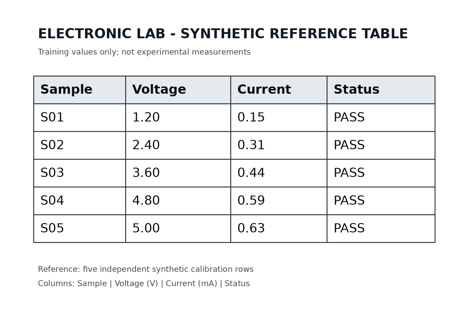
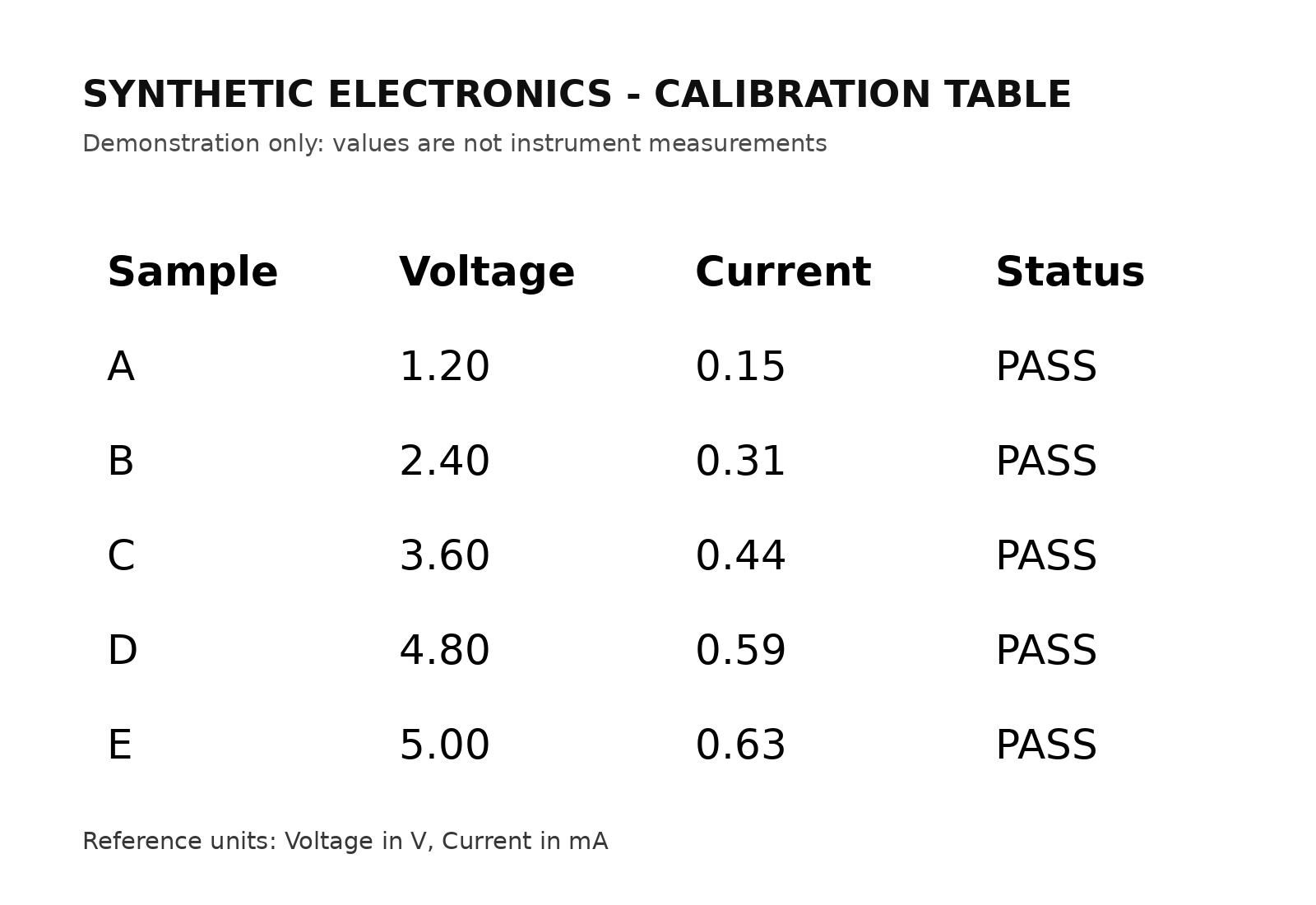
The exercise compares two layouts of a table with sample, voltage, current and state: the first uses a complete grid, the second has well spaced rows and columns without edges.
You can download the image with grid and the gridless version. Both are instructional documents, not photographs of measurements. The difference in layout allows us to observe that a visually clear table for a person can be difficult for an OCR algorithm.
3. Import the source into a Session first
The viewer’s Source selector lists canonical Datasets. Import the image using the standard GX-TXT acquisition module to register it in the Session as an image.raster source.
Opening and publishing are separate operations. the viewer will read the source without altering its bytes and will create, when required, a new Dataset for the table result.
4. Open Unified Documents on the first image
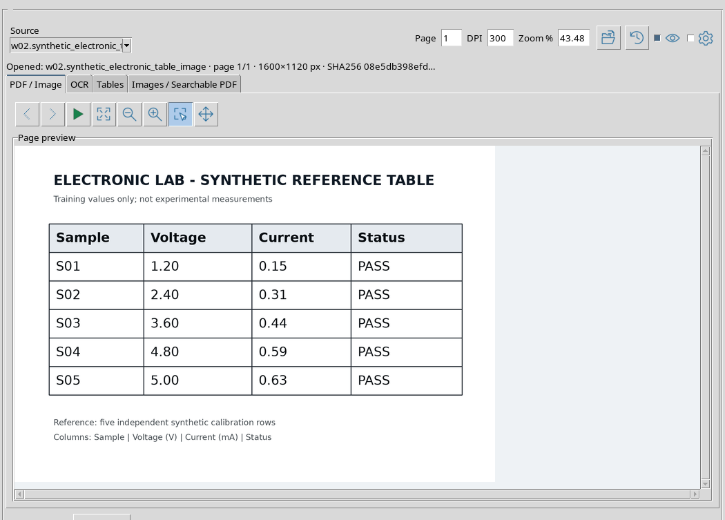
From the Viewers panel of the main window, open Unified Documents, select the first image in Source and press Open source. The PDF / Image tab displays the grid table and its values.
Observe the page number and image size shown in the information bar. A single raster image occupies the 1/1 page.
5. Really define the table with Region
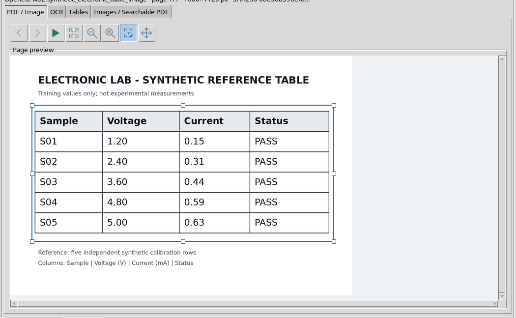
In the PDF / Image tab, activate Region, then mouse trace a rectangle around the table. The selection does not require a prior copy of the file: it defines a region normalized with respect to the source image.
The border must include the header and all the lines we intend to extract. For this first layout, the grid lines are maintained, which form part of the difficulty of recognition.
6. Switch to Tables tab
Select Tables, open Options and set the desired workflow. Table Extractor rebuilds cells using recognized text and its arrangement in space.
Specifying Expected columns = 4 is a reconstruction aid, not an order to manufacture four columns. First row is header signals that the first row will need to be interpreted as a header when publishing the Dataset.
7. First extraction on table with grid
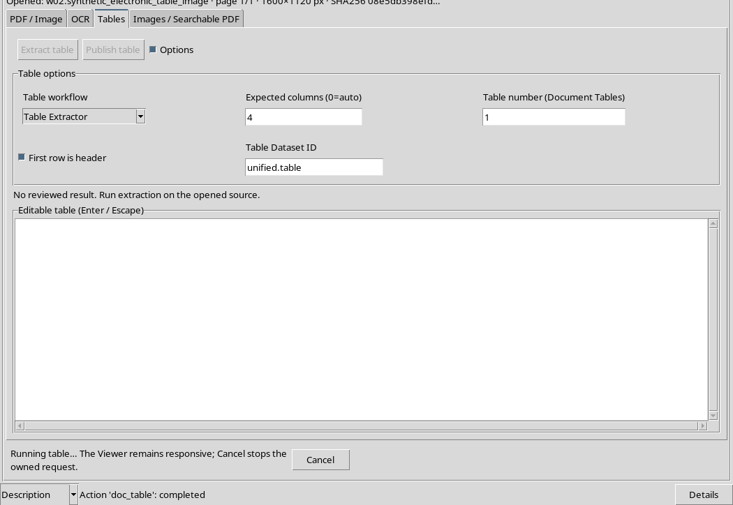
Press Extract table. During processing, temporarily disabled controls and the Cancel button may appear. Wait for conclusion before changing source or changing options.
Extraction is a real operation on the contents of the selected region: it is not enough for the viewer to show the document title to have a usable table.
8. A non-usable result should be declared
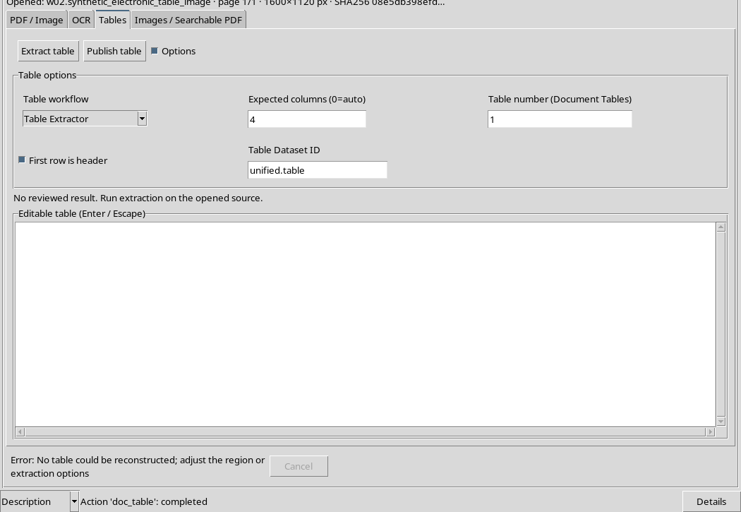
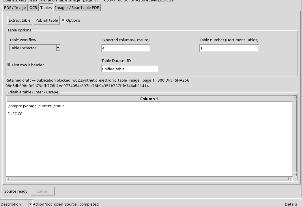
On the first image, Table Extractor does not reconstruct a useful table. the viewer indicates that you need to change the region or options. Even Document Tables failed to get the desired structure: it produced only two rows and one column, not the original scientific matrix.
The result should not be published as representing five measures. It is more correct to correct the way in which the document is presented, or to choose a source that is better suited to the algorithm.
9. Why try a different layout
Optical character recognition and table reconstruction are different tasks. The lines of a grid, font sizes, and the distance between columns can change how the algorithm separates words, cells, and rows.
There is no guarantee that an image with more marked lines will produce a better table. In this exercise we use a second document with more regular spacing. The two images remain different sources, both preserved canonically.
10. Open the second image without grid
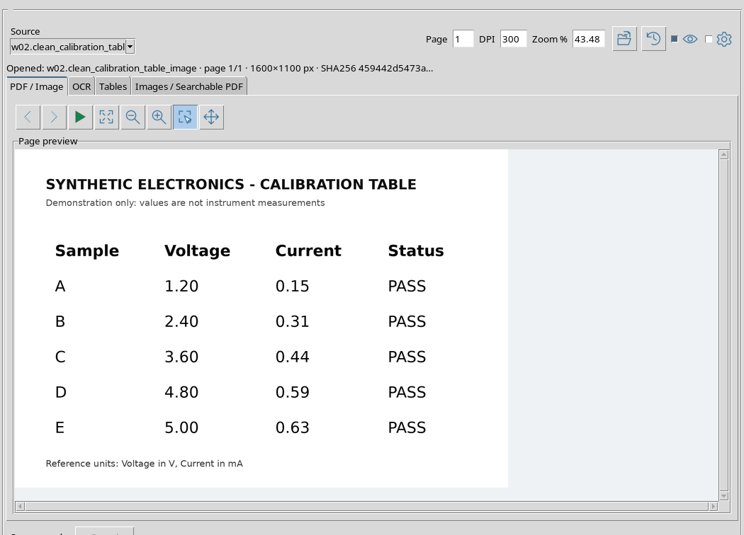
Import the second image as image.raster, update Source, select it and use Open source. The new preview shows the same data categories, with columns separated by blanks.
The document footer explicitly indicates the units of the variables: Voltage in V and Current in mA. This information will be useful in reviewing headers.
11. Select the new ROI accurately
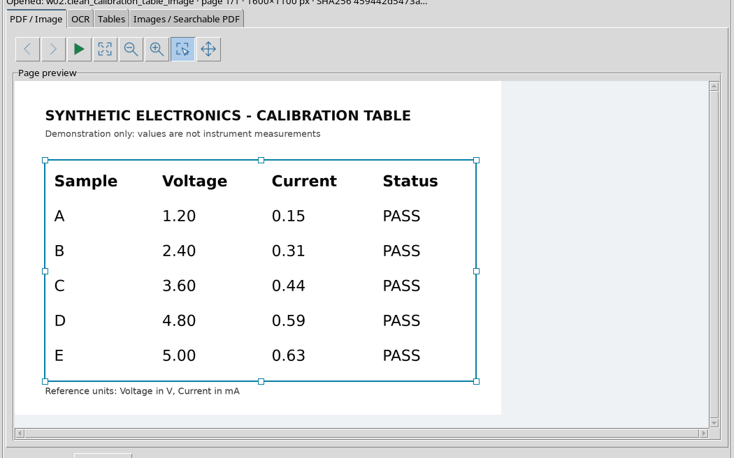
Go back to PDF / Image, activate Region and draw a selection that only includes the header and five rows of the table. It is preferable to exclude the title and final note with the units, which are not tabular cells.
The ROI is expressed in normalized coordinates with respect to the original pixels. Therefore, preview magnification does not change the meaning of the region in the source.
12. Set Table Extractor and Four Columns
On the Tables tab, use Table workflow = Table Extractor, Expected columns = 4 and First row is header enabled. The Table Dataset ID field will be compiled before publication.
In this example Table number does not select a different table: the default value is retained. The expected structure is a row of titles plus five rows of data.
13. Perform recognition on the new source
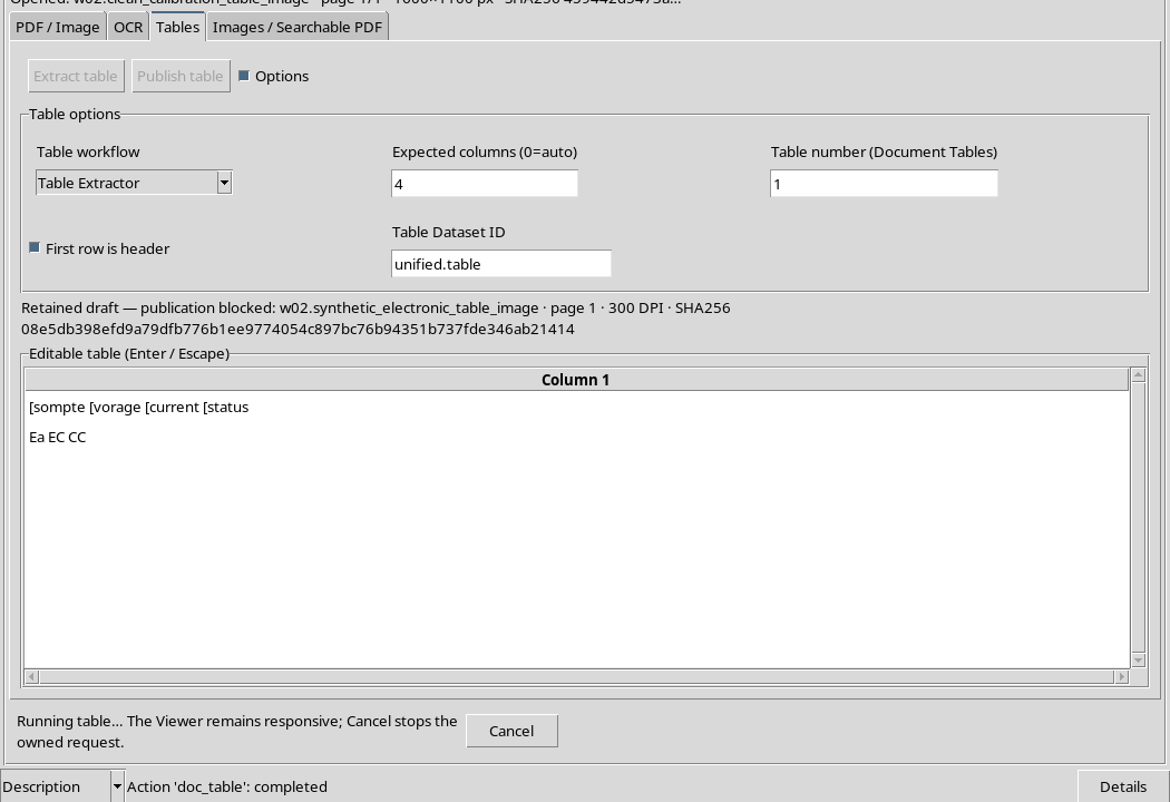
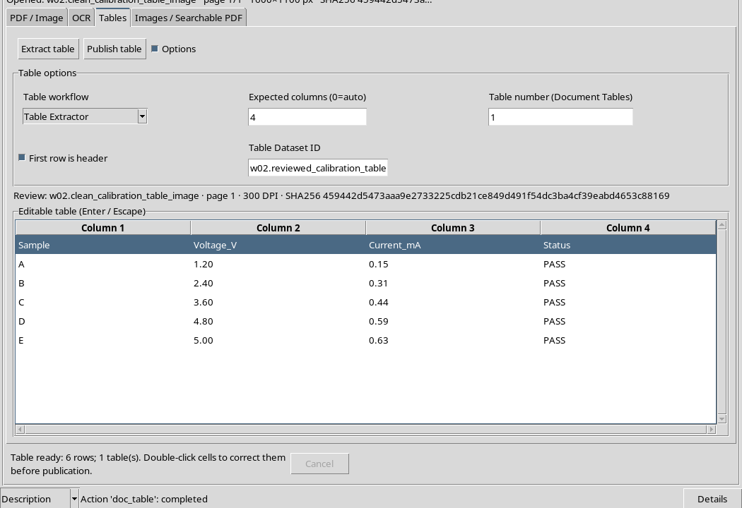
Press Extract table. Recognition is actually performed on the ROI and the result is delivered to the editable grid of the Tables tab.
The presence of the Editable table (Enter / Escape) pane means that the work is still a draft to check: Extract table alone does not create a published canonical Dataset.
14. Compare the six rows and four columns
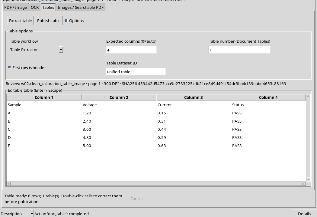
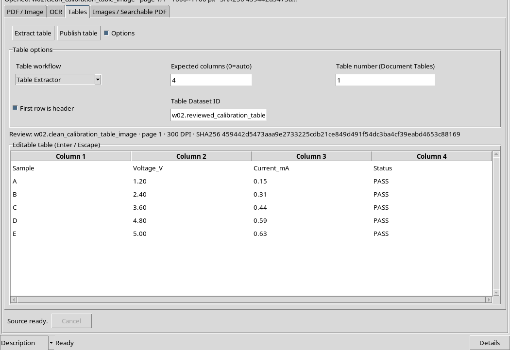
The second extraction returns a matrix of 6 rows × 4 columns, with Sample, Voltage, Current, Status followed by samples A, B, C, D and E.
The comparison with the original table confirms 24 cells on 24: all values, decimal separators, sample letters and PASS indications coincide. This result is specific to the source used: it does not constitute a general measure of OCR accuracy.
15. Check the numeric lines first
The table contains five pairs of voltage and current values. In the teaching document the values are:
| Sample | Voltage (V) | Current (mA) | State |
|---|---|---|---|
| A | 1,20 | 0,15 | PASS |
| B | 2,40 | 0,31 | PASS |
| C | 3,60 | 0,44 | PASS |
| D | 4,80 | 0,59 | PASS |
| E | 5,00 | 0,63 | PASS |
These are five data rows, not six measures: the first row of the matrix is just the header.
16. Integrate units into headers
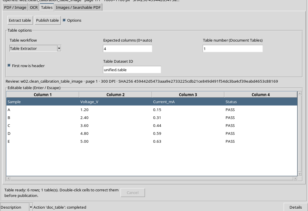
The recognized table text contains the columns Voltage and Current. Because the same image indicates the units in the footer, you can make the headers more informative by editing them in Voltage_V and Current_mA.
This is a reasoned operator correction, not a unit guessed by the OCR. Numbers and other values must remain exactly the same.
17. Edit a cell with the native editor
In the original grid, the double-click opens the cell editor. Edit the content and press Return to confirm. Escape undoes an ongoing edit.
The operation was performed on the two header cells. After confirmation, the matrix includes Sample, Voltage_V, Current_mA, Status and retains all five lines with the recognized values.
18. Why headers count downstream
A visually correct table can still have an unclear structure for those who need to use it in a calculation. An understandable column name allows you to choose the correct variable, and documented units help avoid misinterpretations.
In our example, the annotation of units in the does not equal an automatic physical calibration column name. The Dataset will retain variable names and inferred types; the operator must maintain the meaning of V and mA in subsequent analysis scripts.
19. Choose publication identifier
In the Table Dataset ID field, enter a recognizable name, distinct from the original image Datasets. The identifier should indicate the content or function of the revised table, without overwriting a source.
Before proceeding, still check the open source, the region used, the presence of the correct header and the number of rows.
20. Publish with Publish table
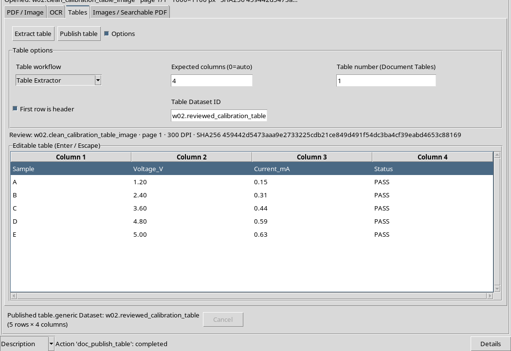
Press Publish table. The action creates a new canonical Dataset table.generic, associated with the image source, page and extraction region.
In the demonstration case the result is a table with five records and four columns. The source images remain available, separated from the published tabular Dataset.
21. What was published
The canonical result preserves the five samples in a CSV table file. Published variables correspond to revised headers, normalized as identifiers: sample, voltage_v, current_ma, status.
The variables voltage_v and current_ma have been interpreted as float64, while sample and status are strings. This verification concerns the actual contract of the published Dataset, not an assumption based only on the appearance of the grid.
22. Independent verification with GX-TXT public APIs
It is useful to check the result with the Public APIs of Canonical Datasets. Reading the contract, variables, respective types and all values allows you to compare the published content with that seen in the GUI and in the original document.
In this example, canonical access confirms the four fields, the five lines and the correspondence of all values. The CSV file also maintains the headers and decimal separators of the revised content.
23. Keep Table Provenance
The published Dataset retains the link to the image.raster source, its SHA-256, page, rendering and normalized region. This allows you to reconstruct which part of the image produced the table.
Do not confuse the result Dataset with the starting image: the CSV does not contain the entire document, but only the extracted and revised data. The two original images have not been modified.
24. Save interface status to Workspace
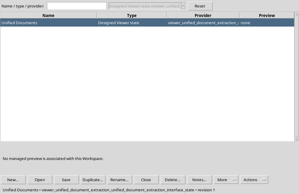
After publishing, use Workspace → Save to preserve the revised table, source, ROI and work context. The Workspace does not replace the published Dataset: its role is to allow the revision to resume.
Then open Session Workspaces… to check that the Workspace Unified Documents is available in the shared framework manager.
25. Close and reopen GX-TXT
Finish the job normally, close the viewer and application, then restart GX-TXT and open the Session itself. The catalog must still contain both images and the published Dataset table.generic.
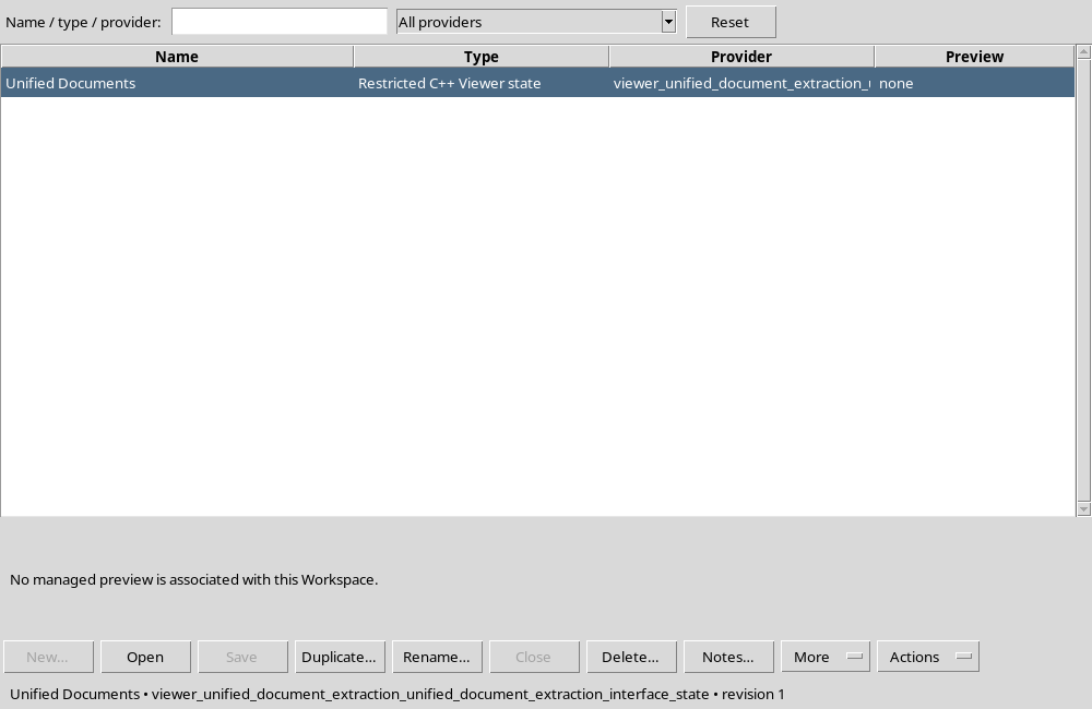
From the Session Workspaces manager, select the saved Workspace and use Open. You do not need to recreate the table or import the file again.
26. Check the recovered table
After re-opening, the Tables card must retain 1 page, the selected area, annotated headers and five sample values.
In this procedure the comparison confirmed that the restored state is identical to the content of the saved Workspace and that the published Dataset remains readable through the canonical APIs.
27. What limits to consider
The first grid image shows that a readable table for a person may not be rebuildable by the OCR. Specifying four columns does not force the creation of four correct columns. The system can return a wrong structure or no table.
Do not publish incomplete or ambiguous results. The most reliable procedure involves comparison with an independent source, human cell review and conservation of units and provenance. In the case of real measurements, any conversion of units or statistical analysis must be carried out at a later stage.
28. Result and continuation
The exercise ends with a revised canonical table, five readable records and four variables, two preserved image sources and a recoverable Workspace after rebooting.
The next chapter completes the path with the publishing images from regions and pages and creating a searchable PDF. The different types of output remain distinct: this allows GX-TXT to preserve provenance and scientific contracts without overwriting the original documents.