

Descriptive statistics
Summarising one or more measurements
Choose analysis.statistics.descriptive. The example compares the location and dispersion of voltage e response. Use guide.descriptive.baseline as the output ID. To reproduce the numbers with the table alone, untick Create group-mean graph. Press Run selected method.
The provider’s initial output ID is statistics.descriptive.summary. The exercise uses a dedicated name.
Configuration in the GUI
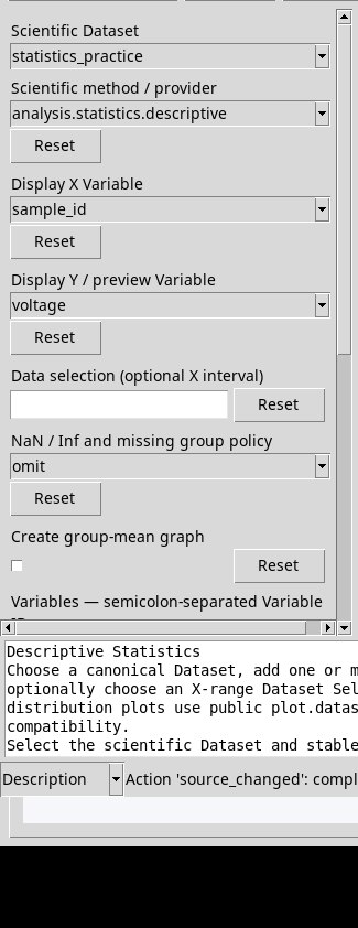
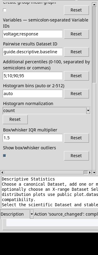
Columns and percentiles
- Variables — semicolon-separated Variable IDs
- Type
voltage;response. Enter the IDs of the numeric columns, in the order in which you want to read the report. A single column is allowed. Each column is processed on its own valid values. - Additional percentiles (0-100, separated by semicolons or commas)
- The initial value is
5;10;90;95. Enter values between 0 and 100, for example25;50;75. The percentiles use type 7 interpolated quantiles. A value such as90requests the ninetieth percentile. An empty list leaves the statistics and the standard quartiles.
Histogram and box plot
- Create group-mean graph
- Tick the box for the histogram and box plot variants, grouped by unit compatibility. The label is shared with ANOVA. Untick it to produce the report and the data without automatic rendering.
- Histogram bins (auto or 2-512)
autoleaves the choice of bins to the renderer. With an integer from 2 to 512, for example6, you make the requested number verifiable and can compare several histograms with the same binning.- Histogram normalization
countshows counts per bin.probabilitydivides each count by the number of observations represented.densityalso divides by the bin width. In the density it is the area of the bars that expresses the mass, and the vertical unit is the inverse of the X unit.- Box/whisker IQR multiplier
- Use a positive value, initially
1.5. The renderer uses Q1 and Q3 plus or minus the IQR multiple to delimit the whiskers. Raising it, for example to2, widens the admissible band. - Show box/whisker outliers
- Leave the box ticked to show the points beyond the whiskers. Untick it to hide those symbols. Use
influenceto check the effect on the extreme value. The option only concerns the plot.
Reading the report
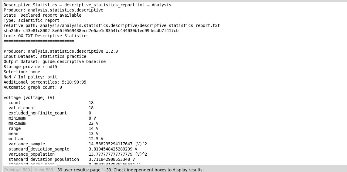
For voltage you get 18 valid values, mean 13 V, median 12.5 V, minimum 8 V, maximum 22 V, Q1 10 V and Q3 15.75 V. The range is 14 V and the IQR 5.75 V. The RMS (about 13.52 V) is the square root of the mean of the squares. Minimum, maximum, percentiles, spread and RMS keep the unit of the measurement; the variance has the squared unit.
The sample standard deviation, about 3.819 V, uses the divisor n − 1 in the variance. The standard deviation of the observed population, about 3.712 V, uses n. The report also gives about 0.900 V as the standard error of the mean, calculated from the sample standard deviation divided by √n. Its sampling interpretation requires independent observations. With a single valid value the sample variance and the standard error are undefined. Check the count, valid and excluded values before interpreting each metric.
In Results search for descriptive_statistics_report.txt o guide.descriptive.baseline. The reusable table lists the metrics per variable with value and unit. Try incomplete to compare omit e error.
Result in the GUI
Plot in Plots
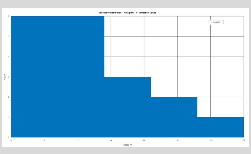
For output IDs, selection and publishing criteria see Options shared by the providers. To look up or open the result go to Tables, reports and plots.