

Principal component analysis
Reducing the dimension of a table
Choose analysis.statistics.pca. In Variables — semicolon-separated Variable IDs enter three numeric IDs voltage;response;influence. Set Missing-pair policy a listwise_omit, centre, standardise and choose two components with count. Use the prefix guide.pca.baseline and, for the reference table, untick the plots.
The provider’s initial output prefix is statistics.pca. The exercise uses a dedicated name.
Configuration in the GUI
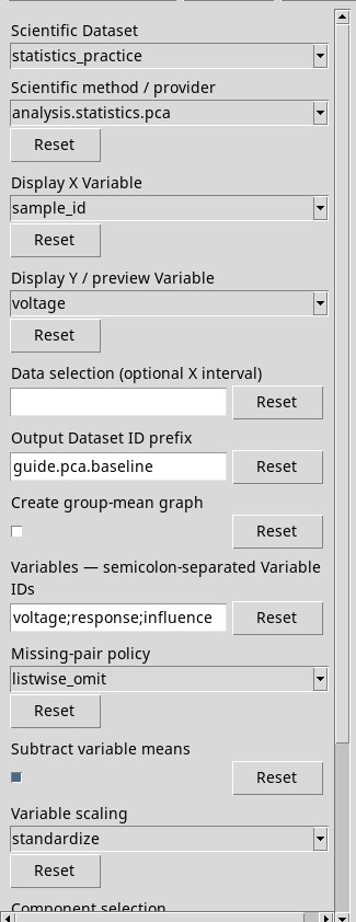
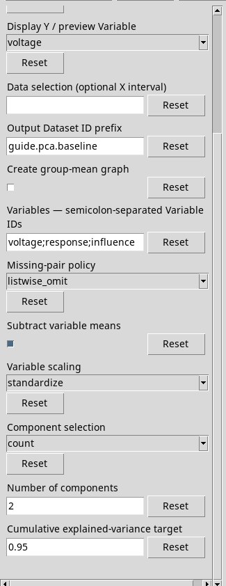
Complete rows, centring and scaling
- Missing-pair policy
listwise_omit(initial) keeps only the complete rows in the chosen columns.errorstops at the first non-finiteness problem. Try addingincomplete. Ifpairwiseelistwiseappear, choose one of the two options allowed for PCA.- Subtract variable means
- The initial tick centres each column. Untick it to study the second moment about the origin. In that case the component quantities are uncentred quadratic magnitudes, to be interpreted relative to the zero fixed for the measurements.
- Variable scaling
standardize(initial) divides each column by the sample standard deviation. It requires positive dispersion and makes the inputs dimensionless, even with mixed linear units.nonekeeps the scale, requires compatible linear units and converts to the first one. For equal units, the non-standardised scale gives more weight to the columns that vary more. Withconstantand standardisation, check the zero-dispersion error.
Choosing how many components to keep
- Component selection, Number of components
- With
countenter an integer. The initial value is 2. Choose a number compatible with the dimensions of the matrix. This parameter determines how many components the projection returns. - Component selection, Cumulative explained-variance target
- With
variance_targetuse a positive fraction up to 1, for example0.95. The method takes the smallest number that reaches the target. The two controls for number and target may remain visible together. The selected mode decides. - Create group-mean graph
- With the box ticked you request the scree plot, the PC1/PC2 score plot when available and the loadings plot. With a single component the PC1/PC2 pair is unavailable.
Reading the decomposition
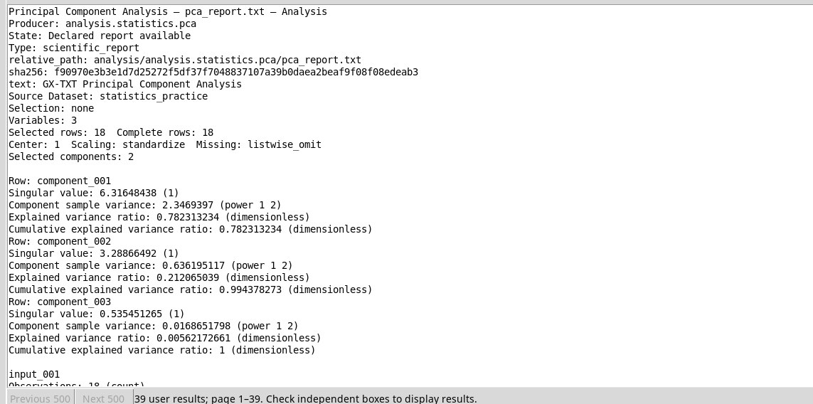
.scores contains the coordinates with the original source_row. .loadings contains the coefficients of the variables in the directions found. .components contains singular values, component moments and individual and cumulative ratios. .scaling records the IDs, means and scales used. In the report the first two components explain about 78.23% and 21.21%, for about 99.44% cumulative. The third appears in the reported spectrum, while the requested scores are two.
The loadings describe directions, with the sign fixed to make the presentation reproducible. Components with equal singular values may admit equivalent bases. Interpret the spectrum in the light of the centring, the units and the excluded data. The analysis explains the variability of the chosen columns and does not provide a significance test.
Result in the GUI
Plot in Plots
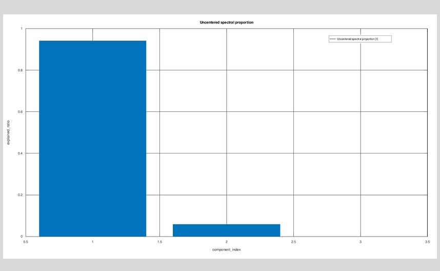
For output IDs, selection and publishing criteria see Options shared by the providers. To look up or open the result go to Tables, reports and plots.