

Empirical distribution
Counting and locating the values
Choose analysis.statistics.distribution. Set Numeric variable to voltage, Explicit bin rule to count, Bin count (count mode) to 6 and the prefix to guide.distribution.baseline. Untick Create group-mean graph for the numeric run. With the box ticked the provider requests the histogram and the ECDF.
The provider’s initial output prefix is statistics.distribution. The exercise uses a dedicated name.
Configuration in the GUI
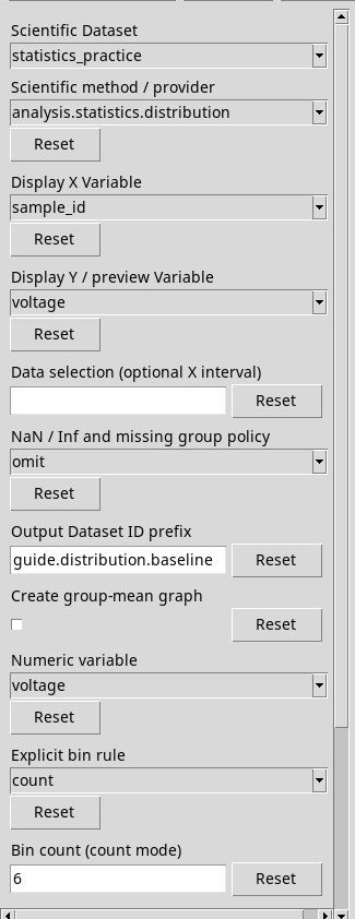
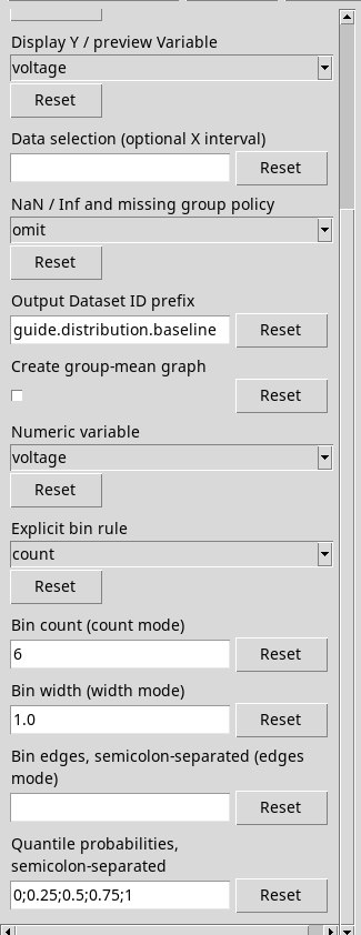
Bin rules
- count and Bin count (count mode)
- Uses an integer number of equal intervals over the range of the finite data. The initial value is 10. The other two interval definitions are inactive for this calculation.
- width and Bin width (width mode)
- Uses a positive width in the units of X. The initial value is 1. Try
3forvoltagein V. The last interval covers the observed maximum. - edges and Bin edges, semicolon-separated (edges mode)
- Write at least two edges in strictly increasing order, for example
8;12;16;20;25. The last edge belongs to the last bin. With edges that cover only part of the distribution read Outside bins. A decreasing list or one with duplicates prevents the processing. - Quantile probabilities, semicolon-separated
- Enter probabilities in the interval [0, 1]. The initial value is
0;0.25;0.5;0.75;1. Try0.1;0.5;0.9to estimate the tenth percentile, the median and the ninetieth percentile. Use the decimal point.
Reading three complementary Datasets
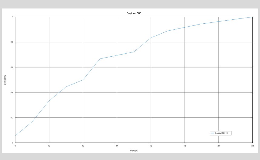
.bins contains edges, centres, counts and frequencies. The relative and cumulative frequencies in any case use all valid observations as the denominator. .ecdf lists the 11 distinct support values of voltage in the example and the fraction of observations less than or equal to each value. .quantiles returns the estimated position for the requested probabilities, using type 7 interpolation and regardless of the bin rule.
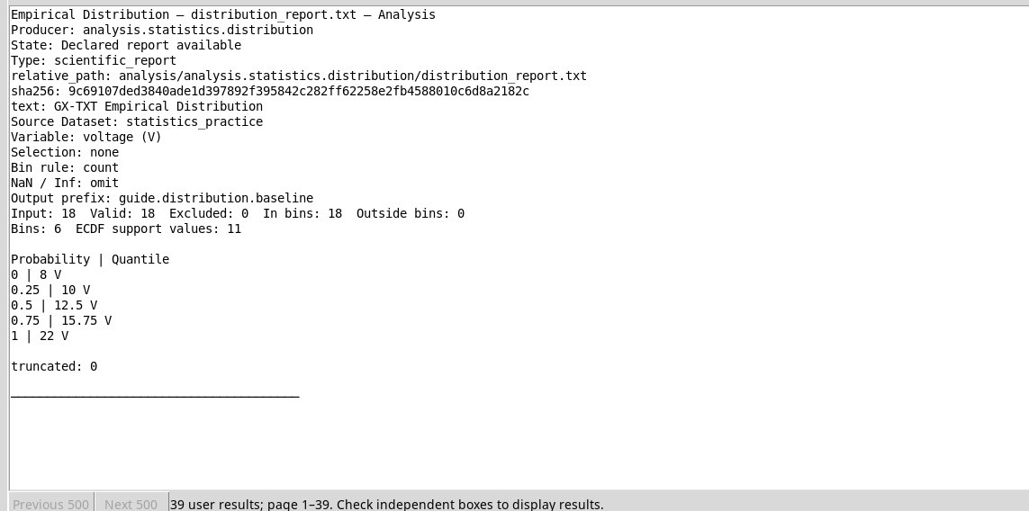
In the report distribution_report.txt, 18 valid rows fall into the 6 bins and the initial probabilities give 8, 10, 12.5, 15.75 and 22 V. The ECDF has a dimensionless Y axis between 0 and 1 and remains defined even if some values fall outside the edges chosen for the histogram.
Result in the GUI
Plot in Plots
For output IDs, selection and publishing criteria see Options shared by the providers. To look up or open the result go to Tables, reports and plots.