OpenFOAM: MRF and the frozen rotor, comparison methods

Deep dive linked to Guide 15 — rotating machinery, MRF and fans of the Learning OpenFOAM 14 path. The article was built by querying a research notebook loaded with the cited sources (open-access papers, theses and technical pages, the OpenFOAM 14 source and Guide 15) and then checking every number against the original sources; the video at the top summarises the same path.

What this is about. This deep dive grows out of Guide 15 and answers a precise question: when is an MRF (“Multiple Reference Frame”) solution of an impeller or rotor reliable, and which methods should it be compared with. It starts from the equations OpenFOAM 14 actually solves, retraces the history of impeller models in stirred vessels (measured boundary conditions, MRF, inner–outer, sliding grid, snapshot), moves on to the turbomachinery tools (mixing plane, harmonic balance) and to the recent literature on RANS, LES and MRF-zone sensitivity, and ends with a verification protocol applicable to the mixerVessel2DMRF tutorial. Sources are cited precisely; where the sources do not say something, we state it.

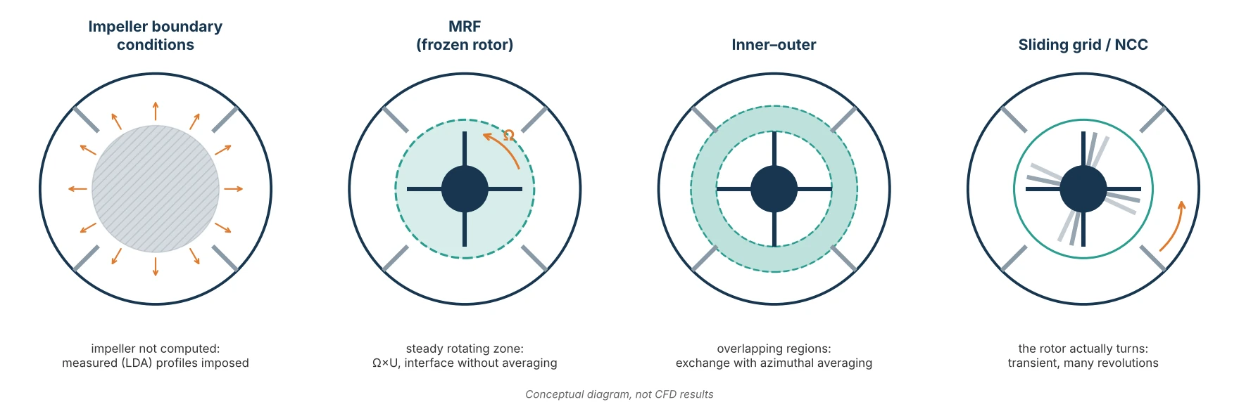
1. The problem: an impeller moving inside a vessel at rest

In a stirred vessel, a pump or a fan, part of the geometry rotates and the rest is stationary. The relative motion of blades and baffles (or stator blades) makes the flow periodic in time, with the blade-passing period. Resolving this flow literally requires a transient computation with a moving mesh, over many revolutions: expensive. All the methods in this article are different compromises between fidelity and cost, and they differ above all in what they do at the interface between the rotating and the stationary part.

2. What OpenFOAM 14 solves in an MRF zone

OpenFOAM uses the absolute-velocity formulation: the U field written to the time directories is always the velocity in the stationary frame, also inside the rotating zone. In the source (MRFZone.C) rotation enters in two places: the Ω × U term added to the material derivative in the cells of the cellZone only, and the correction of the face fluxes, made relative by subtracting (Ω × (C_f − origin)) · S_f.

dU/dt + div(U_r U) + Omega x U = -grad(p) + div(nuEff (grad(U) + grad(U)^T))      in the MRF cellZone
dU/dt + div(U U)                 = -grad(p) + div(nuEff (grad(U) + grad(U)^T))      elsewhere
div(U) = 0,    U_r = U - Omega x (r - origin),    Omega = omega * axis/|axis|

The centrifugal term does not appear separately: in the absolute formulation Ω × U contains both the Coriolis and the centrifugal effects of the relative frame. Walls rotating with the zone use MRFnoSlip, which imposes the absolute velocity Ω × r; if no patch of the U field has an MRF condition, the solver stops.

What “frozen rotor” means. The solution is steady and the blades stay in a single position relative to the baffles for the whole computation. The result is not the average over one revolution but a snapshot for that relative position, computed as if the flow seen by the impeller were steady. At the interface the absolute velocity passes from one zone to the other without circumferential averaging: the approximation is good where the field varies little around the circumference, poor where the interface cuts through jets, blade wakes or vortices.

3. Before MRF: impeller boundary conditions

The first stirred-vessel computations did not compute the impeller. The region swept by the blades was a “black box” and velocity profiles and turbulence quantities measured by laser anemometry (LDA) were imposed on its boundary. The cost is low, but the result depends entirely on the data: Brucato et al. (1998) show that the method gives satisfactory results only if the near-impeller data are known with good accuracy, and can give large errors otherwise.

Luo, Issa and Gosman (1994) proposed “multiple frames of reference” precisely to free the computation from experimental data: with MRF, geometry and rotational speed are enough. This is the scheme OpenFOAM implements with MRFProperties.

4. Inner–outer: two overlapping regions and an average

In the inner–outer approach, compared by Brucato et al. (1998), the vessel is divided into two concentric, partially overlapping regions. The inner region, containing the impeller, is solved in the rotating frame; the outer one in the stationary frame. Both are steady and iteratively exchange boundary conditions along the overlap band, after azimuthal averaging and the transformation for the relative motion.

	MRF	inner–outer
Regions	two, with a single interface	two, with an overlap band
Rotating frame	impeller zone	inner region
Exchange between regions	direct, without averaging	iterative, azimuthally averaged values
Dependence on blade position	yes (frozen rotor)	removed by averaging
Blade wakes in the outer region	yes, for the frozen position	lost by averaging

The two strategies are close relatives; the difference lies in what one accepts to lose: MRF loses the time history, inner–outer also loses the circumferential structure in the outer zone.

5. Sliding grid: the rotor actually turning

With the sliding grid (“sliding mesh”) the mesh block containing the impeller physically rotates at each time step and slides along the cylindrical interface with the stationary block. The computation is transient and requires no experimental data. Two quantitative examples help to understand its cost.

• Bakker, LaRoche, Wang and Calabrese (1998), laminar flow: vessel T = 0.3 m, four-blade 45° pitched-blade turbine, D = T/3, off-bottom clearance C = T/3, blade width 0.2D, four baffles T/12 wide set T/72 off the wall. 90° sector with cyclic conditions, about 49,000 nodes, time step 0.01 s, up to 1000 steps (37.5 revolutions), about 15 minutes of computation per revolution on a Cray C-90. The periodic state needs about 15 revolutions at Re = 40 and about 35 revolutions at Re = 1200; the mean tangential velocity is the slowest quantity to converge. At Re ≈ 40 the impeller stream is mainly radial; above Re ≈ 400 it becomes axial and reaches the bottom; the pumping number decreases significantly as Re decreases.
• Hartmann et al. (2004), Rushton turbine at Re = 7300 (T = 150 mm, D = T/3, N = 2672 rpm, tip speed 7 m/s, silicone oil ρ = 1039 kg/m³, μ = 15.9 mPa·s), transient RANS with sliding grid and SST model in CFX: 241,464 nodes, 228,096 hexahedra, a 1.25 ms step (20° of rotation) to reach the settled regime and then 250 μs (4°), 10 iterations per step, six processors.

The comparison with LDA measurements of a Rushton turbine is also discussed by Ng et al. (1998). The sliding grid is the natural reference to judge MRF, but it must be averaged over an integer number of revolutions after the initial transient, which at low Re can take tens of revolutions.

6. Snapshot: an instant without moving the mesh

The “snapshot” approach of Ranade and Dommeti (1996), extended to impellers of any shape by Ranade, Tayalia and Krishnan (2002), computes a quasi-steady flow for an instantaneous impeller position: in the region swept by the blades time derivatives are written as spatial derivatives, and the impeller is represented by source terms on the blade surfaces. No experimental data or adjustable parameters are needed; in the 2002 work (FLUENT, standard k-ε, QUICK scheme with SUPERBEE limiter) the approach reproduces the pair of trailing vortices behind the blades of a Rushton turbine and of a pitched-blade turbine. Conceptually it is another form of “frozen rotor”, with a different formulation of the impeller zone.

7. The systematic comparison: Brucato et al. (1998) and Micale et al. (1999)

Brucato, Ciofalo, Grisafi and Micale (1998) compared impeller boundary conditions, inner–outer and sliding grid on baffled vessels stirred by one or two Rushton turbines and by an axial helical impeller, against literature data. Conclusion: the first method is reliable only with accurate near-impeller data; inner–outer and sliding grid give satisfactory results without empirical information, with much greater generality.

Micale, Brucato, Grisafi and Ciofalo (1999) applied the same approaches to a vessel with two Rushton turbines on the same shaft. Measurements show that the structure of the circulation loops depends on the impeller positions. Sliding grid and inner–outer give similar results and reproduce this dependence; conditions imposed from single-impeller measurements fail, because the interaction between the two impellers changes the near-blade profiles.

8. RANS versus LES: what an isotropic turbulence model does not see

Hartmann et al. (2004) compared with LDA measurements the transient RANS of section 5 and a lattice-Boltzmann LES: uniform grid of 240³ cells (spacing T/240 = 0.625 mm, impeller of 80 lattice spacings), time step of about 7.74 μs (2900 steps per revolution), about 1.16 GB of memory, averages over 15 revolutions. Main results:

• both computations reproduce the two main mean circulation loops;
• RANS systematically underpredicts the turbulent kinetic energy in the impeller stream, where most of the mixing happens; LES reproduces its structure and width better;
• RANS gives higher and more concentrated dissipation;
• the anisotropy-tensor analysis shows nearly isotropic turbulence in the circulation loops but strongly anisotropic turbulence in the impeller stream, the boundary layers and the separation points: the most likely reason why isotropic eddy-viscosity models fail precisely where turbulence matters most.

For LES of Rushton turbines the earlier reference is Derksen and Van den Akker (1999).

9. Before judging a model: numerical uncertainty and MRF zone size

Coroneo, Montante, Paglianti and Magelli (2011) show that many negative judgements on RANS in stirred vessels stem from insufficient grids and diffusive schemes: before attributing an error to the turbulence model, numerical uncertainty (grid, schemes) must be quantified and the results validated, in their case also with homogenisation curves measured by planar laser-induced fluorescence (PLIF).

Reid et al. (2025), with OpenFOAM and steady MRF on a Rushton turbine at Re = 28,830, varied the MRF zone diameter between 1.10 and 1.93 impeller diameters (constant thickness equal to 1.55 blade heights W):

• velocity profiles change little;
• the power number rises by more than 10 % from the smallest zone to the second one;
• the larger zones create a band of artificial turbulence at the interface; from the smallest to the largest zone the turbulence intensity increases gradually, up to 19 % according to the authors;
• the mixing time of a passive scalar changes by up to a factor of three.

Their recommendation is explicit: the MRF zone-size test should become standard practice in RANS stirred-vessel simulations.

10. From turbomachinery: mixing plane and harmonic balance

In multistage turbomachinery the problem is the same, with blade rows moving relative to each other. Two classic solutions:

• Mixing plane (Denton 1992): at the rotor–stator interface the flow is circumferentially averaged; each blade row is computed steadily in its own frame. It removes the dependence on the relative blade position (like inner–outer), at the price of losing wakes and unsteady interactions.
• Harmonic balance (Hall, Thomas and Clark 2002): the periodic flow is represented by a Fourier series of a few harmonics with spatially varying coefficients, solved as a steady problem with steady-solver techniques; the authors report costs one to two orders of magnitude lower than a time-domain computation.

11. In OpenFOAM: MRF, moving mesh and non-conformal interfaces

In OpenFOAM Foundation, real relative motion is obtained with a moving mesh and non-conformal couplings (NCC), introduced into OpenFOAM-dev on 18 May 2022 and available since OpenFOAM 10, developed by Will Bainbridge with Henry Weller. According to CFD Direct, NCC replaces ACMI and Repeat AMI: AMI interpolation does not guarantee conservative fluxes and in a closed vessel produced a spurious pressure rise of about 40 kPa above the initial 100 kPa; ACMI is reliable only on perfectly flat patches. NCC projects one patch onto the other and creates new faces from the intersections, which belong to both meshes: the coupling stays conservative.

Method	OpenFOAM 14 tutorial
MRF	incompressibleFluid/mixerVessel2DMRF, incompressibleFluid/simpleRushtonMRF
moving mesh with NCC	incompressibleFluid/mixerVessel2D, incompressibleFluid/simpleRushtonNCC, incompressibleFluid/propeller, incompressibleFluid/impeller
single rotating frame (SRF)	incompressibleFluid/rotor2DSRF, incompressibleFluid/mixerSRF
actuator disk	incompressibleFluid/rotorDisk

12. The case study: mixerVessel2DMRF

The Guide 15 tutorial is a 2-D vessel of radius 0.1 m with a 0.02 m hub, four rotor blades up to 0.05 m and four stator blades from 0.07 to 0.1 m, depth 0.01 m, 3072 cells (1536 in cellZone rotor), k-ε model and ν = 1e-5 m²/s. The MRF zone interface is the r = 0.06 m cylinder: 1 cm from the rotor blade tips and 1 cm from the stator blade tips, i.e. inside the wake region, where the hypothesis of a field varying little around the circumference is weakest. With the 30–60–120 rpm campaign the vessel Reynolds number Re = N D²/ν is 500, 1000 and 2000: a transitional regime, in which the k-ε choice must also be checked.

Verification protocol, always on new copies of the cases:

1. Convergence and balance: stable rotor torque and the sum of rotor and stator torques close to zero (add_monitors.py and mrf_torque.py scripts of Guide 15).
2. MRF zone size: move the interface with the rMid variable of the mesh dictionary, for example to 0.055 and 0.065 m, and compare torque, balance and profiles, as recommended by Reid et al. (2025).
3. Turbulence model: repeat the case with simulationType laminar.
4. Actually rotating rotor: the mixerVessel2D tutorial uses the same mesh with real rotation and NCC; before comparing, align the model (laminar versus k-ε) and the blade condition (movingWallSlipVelocity versus MRFnoSlip), and average over an integer number of revolutions after the transient.

# smaller MRF zone, in a NEW copy (rMid between 0.05 and 0.07)
cp "$FOAM_TUTORIALS/resources/blockMesh/mixerVessel2D" system/blockMeshDict
foamDictionary system/blockMeshDict -entry rMid -set 0.055
blockMesh > log.blockMesh 2>&1 && checkMesh > log.checkMesh 2>&1 && foamRun > log.foamRun 2>&1

If torque and mean profiles change little in tests 2–4, the MRF result is defensible; otherwise it must be presented as an estimate, stating which test calls it into question.

13. Summary: which method for which question

Method	Time	Experimental data	Blade passing	When to use it
impeller boundary conditions	steady	essential	no	only with reliable data for the same geometry
MRF (frozen rotor)	steady	no	no, one position	mean fields and power with weak rotor–stator interaction; check the zone
inner–outer	steady, iterative	no	no, averaged	like MRF, without position dependence
snapshot	steady	no	no, one position	near-blade snapshot at reduced cost
mixing plane	steady	no	no, averaged	multistage turbomachinery, global performance
harmonic balance	periodic	no	yes, by harmonics	periodic unsteady flows at reduced cost
sliding grid / NCC	transient	no	yes	rotor–stator interaction, reference for the others
LES with moving impeller	transient	no	yes, with fluctuations	turbulence in the impeller stream, mixing

14. What the sources do not say

• None of the cited sources gives numbers for the OpenFOAM 2-D vessel: the tests in section 12 are to be done, not already known results.
• The power number per unit depth computed in the 2-D case is not comparable with 3-D literature values (for example N_p ≈ 5 for a Rushton turbine in turbulent flow).
• The affinity laws (Q ∝ N, ΔP ∝ N², P ∝ N³) assume a regime in which the Reynolds number does not matter: they do not automatically hold for the Re = 500–2000 campaign.
• A pressure–flow curve cannot be obtained from an MRF simulation of a closed vessel: domains with inlets and outlets are needed.
• Hartmann et al. (2004) do not report the number of revolutions simulated or the RANS computing time; Reid et al. (2025) do not compare MRF with the sliding grid.

15. References

1. J. Y. Luo, R. I. Issa, A. D. Gosman, “Prediction of impeller-induced flows in mixing vessels using multiple frames of reference”, IChemE Symposium Series 136 (1994) 549–556.
2. A. Brucato, M. Ciofalo, F. Grisafi, G. Micale, “Numerical prediction of flow fields in baffled stirred vessels: a comparison of alternative modelling approaches”, Chem. Eng. Sci. 53 (1998) 3653–3684, doi:10.1016/S0009-2509(98)00149-300149-3).
3. G. Micale, A. Brucato, F. Grisafi, M. Ciofalo, “Prediction of flow fields in a dual-impeller stirred vessel”, AIChE J. 45 (1999) 445–464, doi:10.1002/aic.690450303.
4. A. Bakker, R. D. LaRoche, M.-H. Wang, R. V. Calabrese, “Sliding mesh simulation of laminar flow in stirred reactors”, The Online CFM Book (1998, updated 2000), PDF.
5. K. Ng, N. J. Fentiman, K. C. Lee, M. Yianneskis, “Assessment of sliding mesh CFD predictions and LDA measurements of the flow in a tank stirred by a Rushton impeller”, Trans. IChemE 76A (1998) 737–747.
6. V. V. Ranade, S. M. S. Dommeti, “Computational snapshot of flow generated by axial impellers in baffled stirred vessels”, Chem. Eng. Res. Des. 74 (1996) 476–484.
7. V. V. Ranade, Y. Tayalia, H. Krishnan, “CFD predictions of flow near impeller blades in baffled stirred vessels: assessment of computational snapshot approach”, Chem. Eng. Commun. 189 (2002) 895–922, doi:10.1080/00986440213134.
8. J. J. Derksen, H. E. A. Van den Akker, “Large eddy simulations on the flow driven by a Rushton turbine”, AIChE J. 45 (1999) 209–221, PDF.
9. H. Hartmann, J. J. Derksen, C. Montavon, J. Pearson, I. S. Hamill, H. E. A. van den Akker, “Assessment of large eddy and RANS stirred tank simulations by means of LDA”, Chem. Eng. Sci. 59 (2004) 2419–2432, doi:10.1016/j.ces.2004.01.065.
10. M. Coroneo, G. Montante, A. Paglianti, F. Magelli, “CFD prediction of fluid flow and mixing in stirred tanks: numerical issues about the RANS simulations”, Comput. Chem. Eng. 35 (2011) 1959–1968, doi:10.1016/j.compchemeng.2010.12.007.
11. A. Reid et al., “CFD simulation of a Rushton turbine stirred-tank using open-source software with critical evaluation of MRF-based rotation modeling”, Meccanica 60 (2025) 1613–1637, doi:10.1007/s11012-024-01824-z, open access.
12. J. D. Denton, “The calculation of three-dimensional viscous flow through multistage turbomachines”, J. Turbomach. 114 (1992) 18–26, doi:10.1115/1.2927983.
13. K. C. Hall, J. P. Thomas, W. S. Clark, “Computation of unsteady nonlinear flows in cascades using a harmonic balance technique”, AIAA J. 40 (2002) 879–886.
14. CFD Direct, Non-Conformal Coupling and Using Non-Conformal Coupling.
15. OpenFOAM Foundation 14, MRFZone.C and the mixerVessel2DMRF and mixerVessel2D tutorials.

For the monitoring scripts (torque, angular-momentum balance, power) and the 30, 60 and 120 rpm MRF campaign see Guide 15; for discretisation uncertainty and the Grid Convergence Index see Guide 4.