

OpenFOAM: rotating machinery, MRF and fans
Fifteenth guide of the Learning OpenFOAM 14 path and the third of the “Multiphase and moving systems” module of the advanced course, after those on server and transfers, monitoring and convergence, quantitative analysis with ParaView, verification and validation, parameter sweeps, mesh generation, boundary conditions and models, transient simulations, turbulence and RANS models, heat transfer, conjugate heat transfer, species transport, VOF multiphase flows and porous media. This one tackles rotating machinery: the rotating-frame region (MRF) of the mixerVessel2DMRF stirred vessel, the fan represented as an internal pressure jump (fanPressureJump) in the TJunctionFan T-junction, the units of rpm, ω, flow rate and kinematic pressure, the fan curve, the system curve and the operating point. The deep-dive and practical-tip boxes open with a click: they contain every script and file of the package, the actual data of the two tutorials read from their files, the MRF equations and the fanPressureJump condition read in the OpenFOAM 14 source, the omega units trap, the transient nature of the fan case, a corrected defect in the plotting script, six additional tested scripts (torque, power and flow-rate monitors, angular-momentum balance, operating point with the system parabola and affinity laws, dimensionless profiles, estimates) and linked bibliographic references. The archive with all scripts and files is available for download at the end of the article.
OpenFOAM Practical Guide Series · Windows + Linux Server · ParaView 5.13.2
Level: intermediate–advanced · Release: OpenFOAM Foundation 14 · Format: illustrated tutorial and exercises.
Goal. Understand when to simulate rotating machinery with an MRF cell zone and when to represent a fan by an internal pressure jump. Prepare reproducible runs, measure pressure and flow rate with correct units, verify solutions and analyse the results from Windows.
Method note. Illustrations and illustrative fan-curve data in this guide are not CFD results. The supplied tools are training scripts; actual cases must be validated on an OpenFOAM 14 server.
1. Three representations of rotating equipment
Not every engineering question requires the blades to be resolved. Local blade wakes require a suitable geometry, whereas an overall fan effect in a duct can be represented by a pressure–flow relationship.
| Method | Represents | Good for | Main limitation |
|---|---|---|---|
| MRF (Multiple Reference Frame) | Rotating-frame effects in a stationary cell zone | Preliminary impeller or mixer flow estimates | Does not resolve the actual periodic blade passage |
| Internal fan pressure jump | Integral fan action across an internal surface | Duct networks and flow distribution | No blade-to-blade details |
| Moving/sliding mesh | Real relative motion of rotor and stator | Rotor–stator interaction and transients | Higher numerical complexity and cost |
Optional refresher. MRF is a quasi-steady model; the computational mesh does not physically rotate. It must not be mistaken for a moving-mesh transient simulation.
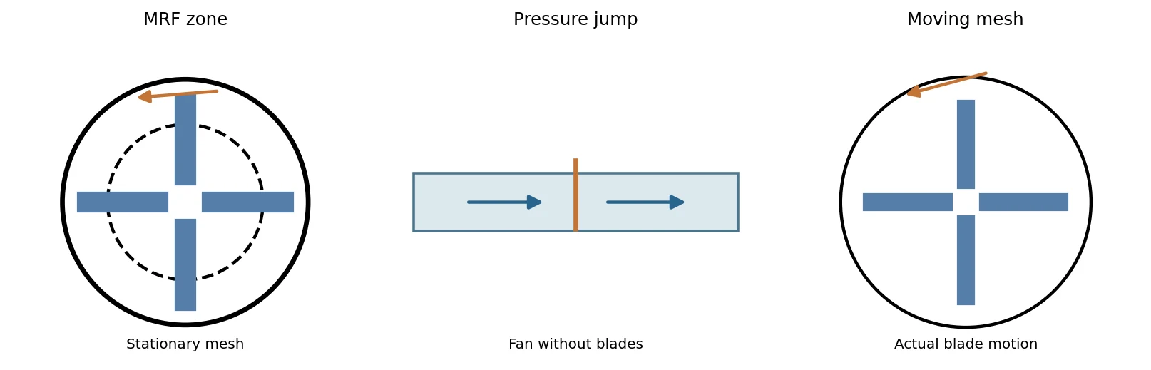
Deep dive · The equations OpenFOAM 14 solves in an MRF zone, read in the source
OpenFOAM uses the absolute-velocity formulation: the U field written to the time directories is always the velocity in the stationary frame, also inside the rotating zone. In the code (MRFZone.C) rotation enters in only two places:
addCoriolisadds the term Ω × U (Coriolis acceleration written for the absolute velocity) to the material derivative, only in the cells of thecellZone;makeRelative(phi)subtracts (Ω × (Cf − origin)) · Sf from the flux of every face of the zone: convection therefore uses the relative velocity Ur = U − Ω × r.
dU/dt + div(U_r U) + Omega x U = -grad(p) + div(nuEff (grad(U) + grad(U)^T))      in the MRF cellZone
dU/dt + div(U U)                 = -grad(p) + div(nuEff (grad(U) + grad(U)^T))      elsewhere
div(U) = 0   (div(Omega x r) = 0, so continuity is the same in both frames)
U_r = U - Omega x (r - origin),   Omega = omega * axis/|axis|
The centrifugal term does not appear explicitly: in the absolute formulation Ω × U contains both the Coriolis and the centrifugal effects of the relative frame. The method remains steady (“frozen rotor”): rotor and stator blades keep a fixed relative position for the whole solution.
Practical tip · All OpenFOAM 14 routes for rotating machinery, with the tutorial to start from
| Method | Foundation 14 tutorial | What it represents |
|---|---|---|
| MRF | mixerVessel2DMRF, simpleRushtonMRF | steady rotating zone, “frozen rotor” |
| SRF | rotor2DSRF, mixerSRF | the whole domain in the rotating frame |
| moving mesh + NCC | mixerVessel2D, simpleRushtonNCC, propeller, impeller | actual blade motion, transient, non-conformal interface |
| actuator disk | rotorDisk | blade forces distributed over a disk |
| pressure jump | TJunctionFan | integral effect of the fan on a surface |
The mixerVessel2D vessel uses the same mesh ($FOAM_TUTORIALS/resources/blockMesh/mixerVessel2D) as the MRF case, with the rotor actually turning: it is the natural comparison to see what MRF loses (see section 10). Non-conformal interfaces (NCC) are described by CFD Direct: Non-Conformal Coupling and Using Non-Conformal Coupling.
Deep dive · MRF and the “frozen rotor” limitation: from Luo et al. (1994) and Brucato et al. (1998) to the comparison methods
What “frozen rotor” means. In an MRF solution the impeller does not move: the equations of the rotating zone are written in the frame attached to the blades (Ω × U term and relative fluxes, first box of this section) and the problem is solved as steady. The rotor blades therefore stay in a single position relative to the baffles and stator blades for the whole computation. The result is not the average over one revolution but a snapshot of the flow for that relative position, computed as if the flow seen by the impeller were steady. At the interface between the two zones the absolute velocity passes from one side to the other without any circumferential averaging: the approximation is good if the field varies little around the circumference there, poor if the interface cuts through blade wakes or jets.
Luo, Issa and Gosman (1994) proposed “multiple frames of reference” for stirred vessels to remove the limitation of the methods then in use, which did not compute the impeller but imposed around it velocities and turbulence measured by LDA (“impeller boundary conditions”). With MRF, geometry and rotational speed are enough: no experimental input. This is the scheme OpenFOAM implements with MRFProperties.
Brucato, Ciofalo, Grisafi and Micale (1998) compared three approaches on baffled vessels stirred by one or two Rushton turbines and by an axial helical impeller, against literature data: (1) impeller boundary conditions derived from measurements; (2) inner–outer, two concentric partially overlapping regions, the inner one solved in the rotating frame and the outer one in the stationary frame, both steady, iteratively exchanging azimuthally averaged values; (3) sliding grid, a transient computation with the inner block actually rotating. Conclusion: method (1) works only if near-impeller data are known with good accuracy and can otherwise give large errors; (2) and (3) give satisfactory results without empirical information. On the dual-impeller vessel (Micale et al. 1999) inner–outer and sliding grid reproduce the dependence of the flow on impeller position, whereas conditions imposed from single-impeller measurements fail. MRF is a close relative of inner–outer: both are steady with a rotating frame, but MRF couples the zones on a single interface without averaging, inner–outer on an overlapping band with azimuthal averaging (which removes the dependence on the frozen position, at the price of losing blade wakes in the outer zone).
| Method | Idea | Time | Experimental data | Blade passing | References |
|---|---|---|---|---|---|
| impeller boundary conditions | impeller not computed, velocity and turbulence imposed around it | steady | yes, essential | no | Brucato 1998 |
| MRF (frozen rotor) | steady rotating zone, interface without averaging | steady | no | no, one position only | Luo 1994; Reid 2025 |
| inner–outer | two overlapping regions, exchange of averaged values | steady, iterative | no | no, averaged | Brucato 1998; Micale 1999 |
| snapshot | quasi-steady flow for one impeller position, time derivatives written as spatial derivatives in the swept region | steady | no | no, one position | Ranade 1996, 2002 |
| mixing plane | circumferential averaging on the rotor–stator interface (turbomachinery) | steady | no | no, removed by averaging | Denton 1992 |
| sliding grid / NCC | the rotor actually turns, non-conformal interface | transient, many revolutions | no | yes | Bakker 1998; Ng 1998; Hartmann 2004 |
| harmonic balance | periodic flow represented by a few Fourier harmonics and solved as a steady problem | periodic | no | yes, harmonics | Hall 2002 |
| LES | large turbulent scales resolved, moving impeller | transient | no | yes, with fluctuations | Hartmann 2004 |
What the more recent literature says. Hartmann et al. (2004) compared, on a Rushton turbine at Re = 7300, a transient RANS with sliding mesh and SST model and an LES: both capture the mean circulation loops well, but RANS systematically underpredicts the turbulent kinetic energy in the impeller stream, where most of the mixing happens. Coroneo et al. (2011) show that many negative judgements on RANS in stirred vessels stem from unverified grids and schemes: numerical uncertainty must be quantified before comparing models. Reid et al. (2025, open access, with OpenFOAM and steady MRF) varied the MRF zone diameter between 1.10 and 1.93 impeller diameters: velocity profiles change little, but the power number rises by more than 10 % between the two smallest zones, the large zones create a band of artificial turbulence at the interface and the mixing time of a passive scalar changes by up to a factor of three. They recommend making the zone-size test standard practice.
What it means for this guide’s vessel. The interface is at r = 0.06 m, 1 cm from the rotor blade tips (0.05 m) and 1 cm from the stator blade tips (0.07 m): rotor and stator are close and the interface lies in the wake region. Two direct tests, in new copies: (a) zone-size sensitivity, moving the interface with the rMid variable of the mesh dictionary (for example 0.055 and 0.065 m; the intermediate blocks adapt automatically) and comparing torque, angular-momentum balance and profiles; (b) comparison with the actually rotating rotor, the mixerVessel2D tutorial on the same mesh, averaged over an integer number of revolutions (section 10). If torque and mean profiles change little in both tests, the MRF result is defensible; otherwise it must be presented as an estimate.
# zone-size test in a NEW copy (rMid must stay between rRotorTip 0.05 and rStatorTip 0.07)
cp "$FOAM_TUTORIALS/resources/blockMesh/mixerVessel2D" system/blockMeshDict
foamDictionary system/blockMeshDict -entry rMid -set 0.055
blockMesh > log.blockMesh 2>&1 && checkMesh > log.checkMesh 2>&1 && foamRun > log.foamRun 2>&1- J. Y. Luo, R. I. Issa, A. D. Gosman, «Prediction of impeller-induced flows in mixing vessels using multiple frames of reference», IChemE Symposium Series 136 (1994) 549–556.
- A. Brucato, M. Ciofalo, F. Grisafi, G. Micale, «Numerical prediction of flow fields in baffled stirred vessels: a comparison of alternative modelling approaches», Chem. Eng. Sci. 53 (1998) 3653–3684, doi:10.1016/S0009-2509(98)00149-3 (record with abstract).
- G. Micale, A. Brucato, F. Grisafi, M. Ciofalo, «Prediction of flow fields in a dual-impeller stirred vessel», AIChE J. 45 (1999) 445–464, doi:10.1002/aic.690450303.
- V. V. Ranade, S. M. S. Dommeti, «Computational snapshot of flow generated by axial impellers in baffled stirred vessels», Chem. Eng. Res. Des. 74 (1996) 476–484; V. V. Ranade, Y. Tayalia, H. Krishnan, Chem. Eng. Commun. 189 (2002) 895–922, doi:10.1080/00986440213134.
- J. D. Denton, «The calculation of three-dimensional viscous flow through multistage turbomachines», J. Turbomach. 114 (1992) 18–26, doi:10.1115/1.2927983.
- A. Bakker, R. D. LaRoche, M.-H. Wang, R. V. Calabrese, «Sliding mesh simulation of laminar flow in stirred reactors», The Online CFM Book (1998, PDF).
- K. Ng, N. J. Fentiman, K. C. Lee, M. Yianneskis, «Assessment of sliding mesh CFD predictions and LDA measurements of the flow in a tank stirred by a Rushton impeller», Trans. IChemE 76A (1998) 737–747.
- K. C. Hall, J. P. Thomas, W. S. Clark, «Computation of unsteady nonlinear flows in cascades using a harmonic balance technique», AIAA J. 40 (2002) 879–886 (record).
- H. Hartmann, J. J. Derksen, C. Montavon, J. Pearson, I. S. Hamill, H. E. A. van den Akker, «Assessment of large eddy and RANS stirred tank simulations by means of LDA», Chem. Eng. Sci. 59 (2004) 2419–2432, doi:10.1016/j.ces.2004.01.065.
- M. Coroneo, G. Montante, A. Paglianti, F. Magelli, «CFD prediction of fluid flow and mixing in stirred tanks: numerical issues about the RANS simulations», Comput. Chem. Eng. 35 (2011) 1959–1968, doi:10.1016/j.compchemeng.2010.12.007.
- A. Reid et al., «CFD simulation of a Rushton turbine stirred-tank using open-source software with critical evaluation of MRF-based rotation modeling», Meccanica 60 (2025) 1613–1637, doi:10.1007/s11012-024-01824-z (open access).
2. Two official Foundation 14 tutorials
We use two distinct cases shipped with OpenFOAM 14:
$FOAM_TUTORIALS/incompressibleFluid/mixerVessel2DMRF: an enclosed vessel with arotorcell zone,constant/MRFPropertiesand rpm-based angular speed. It demonstrates rotation-axis setup and mean flow fields.$FOAM_TUTORIALS/incompressibleFluid/TJunctionFan: a T-junction containing an internal fan surface created byblockMesh,createZonesandcreateBaffles. Thepfield usesfanPressureJump.
They are not interchangeable. In particular, the enclosed MRF mixer has no inlet or outlet, so it cannot directly yield a fan pressure–flow characteristic. The pressure-jump and flow-distribution exercise uses the T-junction; a true resolved-impeller fan curve requires a separate fan geometry and multiple operating points.
Deep dive · The data sheet of the two tutorials, read from their files
| Item | mixerVessel2DMRF | TJunctionFan |
|---|---|---|
| geometry | 2-D vessel of radius 0.1 m; hub 0.02 m; 4 rotor blades up to 0.05 m; 4 stator blades from 0.07 to 0.1 m; rotor/stator interface at r = 0.06 m; depth 0.01 m | inlet duct 0.2 × 0.02 × 0.02 m and two 0.02 × 0.2 m branches towards y = ±0.21 m |
| mesh | 3072 cells (1536 in cellZone rotor), 2.5 mm radially, 96 cells around; zero-thickness blades | 3875 cubic 4 mm cells |
| physics | incompressibleFluid, steady (SIMPLE), RAS k-ε, ν = 1e-5 m²/s | incompressibleFluid, transient (PIMPLE, Euler), RAS k-ε, ν = 1e-5 m²/s |
| control | 500 iterations (deltaT 1), write every 50; relaxation p 0.3, U/k/ε 0.5 | endTime 1.5 s, initial deltaT 1 ms, adaptive with maxCo 3, write every 0.1 s |
| boundaries | rotor MRFnoSlip, stator noSlip, front/back empty; p zeroGradient everywhere with pRefCell 0, pRefValue 0 | inlet uniformTotalPressure p0 from 10 to 40 m²/s² between t = 0 and 1 s, then constant; outlet1 p = 10, outlet2 p = 0; walls noSlip |
| initial values | k = 1 m²/s², ε = 20 m²/s³, U = 0 | fields from *.orig files, U = 0 |
| preparation | blockMesh -dict $FOAM_TUTORIALS/resources/blockMesh/mixerVessel2D | blockMesh, createZones, createBaffles |
Sources: mixerVessel2DMRF, resources/blockMesh/mixerVessel2D, TJunctionFan. Cell counts computed from the dictionary blocks (g15_estimates.py script, section 3).
Practical tip · TJunctionFan is a transient case with a ramped inlet: measure after t = 1 s
The tutorial controlDict is not steady: endTime 1.5, adaptive time step with maxCo 3 and inlet total pressure growing linearly from 10 to 40 m²/s² during the first second (table (0 10) (1 40), constant afterwards). Flow rates and pressures therefore change in time by construction: a measurement taken at t = 0.5 s describes a point of the ramp, not the settled operation. Refer measurements to a window after the ramp (for example 1.2–1.5 s), check that the drift between the two halves of the window is negligible (fan_balance.py does it, section 7) and, if it is not, extend endTime in a new copy.
// 0/p.orig of the tutorial (kinematic pressure)
inlet   { type uniformTotalPressure; p0 table ((0 10) (1 40)); }
outlet1 { type fixedValue; value uniform 10; }
outlet2 { type fixedValue; value uniform 0; }
Deep dive · Why the tutorial has 0/U.orig and 0/p.orig and no 0/U
In OpenFOAM 14, when a file does not exist, reading looks for the compressed .gz version and then for the .orig version (IFstream.C). createBaffles, with fields true, thus reads the starting fields and writes into 0/ complete fields including the new baffle0/1 and fan0/1 patches. The *.orig originals stay intact: to start again a fresh copy of the tutorial is enough, which is exactly what prepare_fan_case.py does.
Practical tip · The non-conformal variant of the tutorial: Allrun-NCC
The same case contains Allrun-NCC: the baffles are created with system/createBafflesDict.NCC and then coupled with createNonConformalCouples. It is a good exercise to learn the command chain also used for moving-mesh rotors (section 10), on a small and fast case. Use it in a separate copy, with its own prefix, so as not to mix results with the reference case.
blockMesh
createZones
createBaffles -dict system/createBafflesDict.NCC
createNonConformalCouples
foamRun
3. Quantities and units: rpm, angular speed, flow and pressure
The relationship between rotational speed n and angular velocity is

The volumetric flow through an oriented surface S is

In the incompressible tutorial cases, p is kinematic pressure, measured in m²/s². Given a known constant density, the physical pressure rise in Pa is ΔP = rho * Δp. Do not label p as Pa. The reference physicalProperties file specifies kinematic viscosity nu; density must be stated separately for physical-pressure conversion.
Sign convention. Surface normals determine the sign of Q. Flow conservation can only be checked when all sections use consistent outward normals.
Deep dive · The numbers of the MRF campaign and of the fan case (g15_estimates.py script)
The stirred-vessel Reynolds number is Re = N D²/ν, with N in revolutions per second and D the impeller diameter (here 2 × 0.05 m). With ν = 1e-5 m²/s the 30–60–120 rpm campaign covers Re = 500–2000: a transitional regime, far from the threshold of about 10⁴ beyond which a stirred vessel is considered fully turbulent. The tutorial k-ε model should therefore be read as a teaching choice, not as a model validated for this regime (see the tip in section 5). The ratio between the initial k (1 m²/s²) and Utip² shows how much the initial turbulence is overestimated: 40 times at 30 rpm.
mixerVessel2D mesh: 3072 cells (1536 in cellZone rotor, 1536 in stator); radial size 2.50 mm; 96 cells around
   rpm    omega   T [s]   U_tip  Re=ND2/nu   Re_tip  N D2 [m2/s]  k0/Utip2
    30   3.1416       2  0.1571        500     1571        0.005      40.5
    60   6.2832       1  0.3142       1000     3142         0.01      10.1
   120  12.5664     0.5  0.6283       2000     6283         0.02      2.53
Stirred-tank practice: laminar Re < ~10, transitional ~10..1e4, fully turbulent Re > ~1e4.

TJunctionFan: duct area 0.0004 m2, fan area 0.000144 m2 (36 % of the section)
  fan jump               dp =    100 m2/s2 -> U_max = sqrt(2 dp) =  14.14 m/s, Re_duct =  2.83e+04
  inlet p0 at t >= 1 s   dp =     40 m2/s2 -> U_max = sqrt(2 dp) =   8.94 m/s, Re_duct =  1.79e+04
  jump + p0 - outlet2    dp =    140 m2/s2 -> U_max = sqrt(2 dp) =  16.73 m/s, Re_duct =  3.35e+04
  jump 100 m2/s2 with rho = 1.2 kg/m3 (air): 120 Pa
  jump 100 m2/s2 with rho = 1000 kg/m3 (water): 100000 Pa
#!/usr/bin/env python3
# SPDX-License-Identifier: GPL-3.0-or-later
"""Order-of-magnitude checks for the two Guide 15 tutorials (OpenFOAM 14).
mixerVessel2DMRF (data from resources/blockMesh/mixerVessel2D and the case):
hub radius 0.02 m, rotor blade tip 0.05 m, rotor/stator interface 0.06 m,
stator blade tip 0.07 m, vessel 0.1 m, slab depth 0.01 m, 4 rotor and 4
stator zero-thickness blades, nu = 1e-5 m2/s, k-epsilon. For each rpm the
script prints omega, the rotation period, the blade-tip speed, the stirred
tank Reynolds number Re = N D^2/nu (N in rev/s, D = rotor tip diameter),
the tip Reynolds number U_tip D/nu, the swept-volume flow scale N D^2 (per
unit depth) and the ratio of the initial k (1 m2/s2) to U_tip^2.
TJunctionFan: duct 0.02 x 0.02 m, fan plate 0.012 x 0.012 m at x = 0.1 m
(9 faces of the 4 mm mesh), kinematic jump 100 m2/s2, inlet total pressure
ramp 10 -> 40 m2/s2 over 0..1 s, outlet1 p = 10, outlet2 p = 0. Upper-bound
velocity sqrt(2 dp) if a kinematic dp were entirely converted to kinetic
energy, its Reynolds number on the 0.02 m duct and the jump in Pa for a few
declared densities.
Theoretical values, not CFD results.
"""
import argparse
import math
R_HUB, R_TIP, R_MID, R_STATOR, R_VESSEL, DEPTH = 0.02, 0.05, 0.06, 0.07, 0.1, 0.01
def mesh_counts():
blade, mid = 12 * 12, 12 * 4 # cells per block (tangential x radial)
rotor = 8 * (blade + mid)
stator = 8 * (blade + mid)
return rotor, stator
def main():
ap = argparse.ArgumentParser(description=__doc__, formatter_class=argparse.RawDescriptionHelpFormatter)
ap.add_argument('--rpm', type=float, nargs='+', default=[30, 60, 120])
ap.add_argument('--nu', type=float, default=1e-5)
a = ap.parse_args()
rot, sta = mesh_counts()
print(f'mixerVessel2D mesh: {rot + sta} cells ({rot} in cellZone rotor, {sta} in stator); '
f'radial size {(R_TIP - R_HUB) / 12 * 1000:.2f} mm; 96 cells around')
D = 2 * R_TIP
print(f"{'rpm':>6s} {'omega':>8s} {'T [s]':>7s} {'U_tip':>7s} {'Re=ND2/nu':>10s} {'Re_tip':>8s} {'N D2 [m2/s]':>12s} {'k0/Utip2':>9s}")
for n in a.rpm:
N = n / 60
w = 2 * math.pi * N
ut = w * R_TIP
print(f'{n:6g} {w:8.4f} {1 / N:7.3g} {ut:7.4f} {N * D * D / a.nu:10.4g} {ut * D / a.nu:8.4g} {N * D * D:12.4g} {1.0 / ut ** 2:9.3g}')
print('Stirred-tank practice: laminar Re < ~10, transitional ~10..1e4, fully turbulent Re > ~1e4.')
print()
A_duct, A_fan = 0.02 * 0.02, 0.012 * 0.012
print(f'TJunctionFan: duct area {A_duct:.4g} m2, fan area {A_fan:.4g} m2 ({100 * A_fan / A_duct:.0f} % of the section)')
for label, dp in (('fan jump', 100.0), ('inlet p0 at t >= 1 s', 40.0), ('jump + p0 - outlet2', 140.0)):
u = math.sqrt(2 * dp)
print(f' {label:22s} dp = {dp:6g} m2/s2 -> U_max = sqrt(2 dp) = {u:6.2f} m/s, Re_duct = {u * 0.02 / a.nu:9.3g}')
for rho, name in ((1.2, 'air'), (1000, 'water')):
print(f' jump 100 m2/s2 with rho = {rho:g} kg/m3 ({name}): {100 * rho:g} Pa')
return 0
if __name__ == '__main__':
main()Practical tip · Which density to declare: the fan case is “air”, the mixer is not
- ν = 1e-5 m²/s is close to that of air at 20 °C (about 1.5e-5): for TJunctionFan the consistent choice is ρ ≈ 1.2 kg/m³, so the 100 m²/s² jump is about 120 Pa and the final inlet total pressure 48 Pa.
- For a liquid, ν = 1e-5 m²/s corresponds to a fluid ten times more viscous than water (for example a light oil). Declare the ρ of the fluid you intend to represent and write it in the
rho_kg_m3column ofmeasurements_template.csv. - The same number 100 would become 100,000 Pa in water: this is why the guide insists on not labelling
pin pascals.
Deep dive · Signs of flow rates in OpenFOAM: outward normal and patchFlowRate functions
On boundary patches the area vector Sf always points out of the domain, so the flux phi is positive when leaving and negative when entering. The patchFlowRate function sums phi over the faces: Qin comes out negative, Qout1 and Qout2 positive, and their sum is the mass-balance residual. In ParaView slices the normal is chosen by the user instead: this is why the guide asks to declare the orientation.
4. Inside an MRF region
The reference mixerVessel2DMRF case contains:
MRF
{
    cellZone    rotor;
    origin      (0 0 0);
    axis        (0 0 1);
    omega       60 [rpm];
}
The rotor name must match an actual mesh cellZone. origin is a point on the axis; axis sets its direction. The Foundation 14 tutorial uses the unit-bearing omega entry [rpm]. In 0/U, the rotating wall uses MRFnoSlip, whereas the stationary wall uses noSlip. The case runs foamRun with solver incompressibleFluid in steady-state mode.
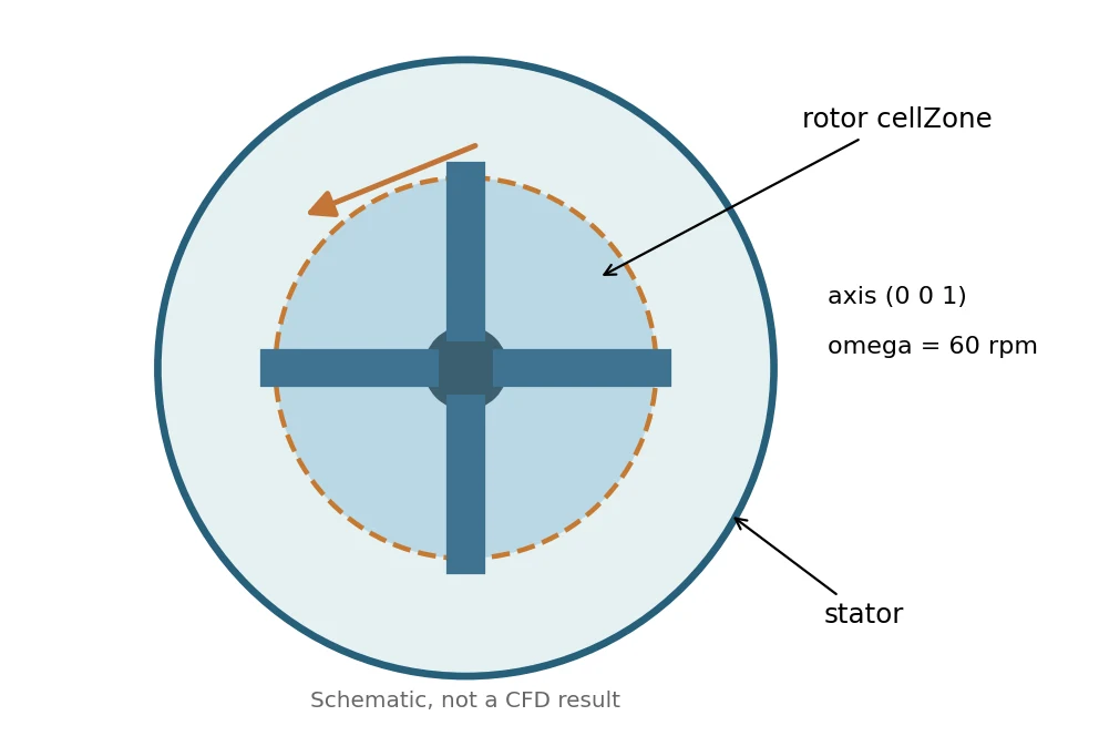
Before running: check foamVersion, inspect MRFProperties, use the shared $FOAM_TUTORIALS/resources/blockMesh/mixerVessel2D mesh dictionary, run checkMesh, then inspect the rotor cell zone in ParaView.
Deep dive · omega, rpm and units: the “omega 60;” trap
The angular speed is read by the Function1s::omega class, which accepts three equivalent forms and a function of time:
omega   6.28319;      // default units: rad/s
omega   60 [rpm];     // explicit unit conversion (tutorial syntax)
rpm     60;           // backward compatible, default units rpm (may be removed)

omega table ((0 0) (2 6.28319)); // ramp in rad/s, read at each time/iteration- Beware:
omega 60;without units means 60 rad/s, i.e. about 573 rpm, almost ten times the intended speed. - If both
omegaandrpmare present the solver stops with “Rotational speeds rpm and omega both defined”; if neither is present, with “Neither rotational speed rpm nor omega defined”. - The sign follows the right-hand rule about
axis: withaxis (0 0 1)and positive ω the rotation is counter-clockwise seen from +z. The axis is normalised by the code, so(0 0 2)is the same as(0 0 1). - An ω ramp (table) is useful to start a difficult steady computation; the final value is the one to report with the results.
Deep dive · What MRFnoSlip does and which faces rotate
MRFnoSlip(source) imposes on the wall the absolute velocity Ω × (r − origin): the wall is at rest in the rotating frame, i.e. no slip for the fluid rotating with it.- At start-up the code checks that at least one patch of the U field has an MRF condition; otherwise it stops with “Walls rotating in the MRF region should have the MRFnoSlip boundary condition”. With several MRF zones the zone is given with
MRFZoneName. - In OpenFOAM 14 the MRF region contains every internal face with at least one cell in the zone and every boundary face of zone cells (
setMRFFaces). The flux is made relative only where the condition does not fix the value: on walls the boundary condition decides. A stationary wall inside the rotating zone is treated withnoSlip, which in the absolute formulation really means stationary. - The zone interface must be a surface of revolution about the axis (here the r = 0.06 m cylinder generated by the blocks): only then does the fluid crossing it not “see” a moving edge.
Practical tip · The #print line of the tutorial and the log check
The original MRFProperties also contains, after omega, the #print directive (omitted in the guide listing): it prints the dictionary as read into the log. After the run, searching for it is enough to verify the zone, axis and speed actually used.
grep -n -A8 "^MRF" log.foamRun        # dictionary echoed by #print
foamDictionary constant/MRFProperties -entry MRF/omega
grep -c rotor constant/polyMesh/cellZones  # the zone exists after blockMesh
5. Exercise A — Three-speed MRF campaign
Create three independent tutorial copies at 30, 60 and 120 rpm. The installed tutorials are never modified.
After transferring the supplied scripts folder to Linux, initialize OpenFOAM 14 in the shell:
foamVersion
python3 scripts/prepare_mrf_cases.py --dest "$HOME/OpenFOAM/guide15_MRF" --rpm 30 60 120
bash scripts/run_mrf_case.sh "$HOME/OpenFOAM/guide15_MRF/mrf_0060rpm"
Only one case is run by the last command. Inspect the 60 rpm result and its logs first, then run the other cases. The wrapper runs blockMesh using the official shared dictionary, checkMesh and foamRun, with separate logs. Existing solver logs and simulation results are never automatically removed or overwritten.
Record: mesh cell count, mesh quality, final residuals, peak and region-averaged velocities, recirculation and machine time. Do not misinterpret mixer velocities as a fan performance curve.
Deep dive · Package script: prepare_mrf_cases.py
It copies the installed tutorial into a new directory for each speed and changes a single line of MRFProperties: it looks exactly for omega 60 [rpm]; and replaces it, stopping if the tutorial syntax is not the expected one (a useful safeguard should an OpenFOAM update change the file). It refuses existing destination directories, duplicate or non-positive speeds and accepts integer rpm only. Tested on the OpenFOAM 14 tutorial: the comparison with the original shows only the omega line changed and the GUIDE15_CASE.txt file added; a second run on the same destination is refused.
#!/usr/bin/env python3
# SPDX-License-Identifier: GPL-3.0-or-later
"""Create non-overwriting OpenFOAM 14 MRF training cases from the installed tutorial."""
from __future__ import annotations
import argparse
import os
from pathlib import Path
import re
import shutil
import sys


def main() -> int:
    parser = argparse.ArgumentParser(description=__doc__)
    parser.add_argument('--dest', type=Path, required=True, help='New campaign directory')
    parser.add_argument('--rpm', type=int, nargs='+', default=[30, 60, 120])
    args = parser.parse_args()
    if any(x <= 0 or x > 100000 for x in args.rpm) or len(set(args.rpm)) != len(args.rpm):
        parser.error('rpm must be distinct positive integers <= 100000')
    tutorial_root = os.environ.get('FOAM_TUTORIALS')
    if not tutorial_root:
        parser.error('FOAM_TUTORIALS is missing: source the OpenFOAM 14 environment')
    source = Path(tutorial_root) / 'incompressibleFluid' / 'mixerVessel2DMRF'
    mrf_file = source / 'constant' / 'MRFProperties'
    if not mrf_file.is_file():
        parser.error(f'Missing Foundation 14 tutorial source: {mrf_file}')
    source_text = mrf_file.read_text(encoding='utf-8')
    pattern = r'(?m)^(\s*omega\s+)60(\s+\[rpm\]\s*;)'
    if len(re.findall(pattern, source_text)) != 1:
        parser.error('Reference MRFProperties differs from expected Foundation 14 syntax')
    destination = args.dest.expanduser().resolve()
    if destination.exists():
        parser.error(f'Refusing to overwrite existing destination: {destination}')
    destination.mkdir(parents=True)
    for rpm in args.rpm:
        name = f'mrf_{rpm:04d}rpm'
        target = destination / name
        shutil.copytree(source, target)
        new_text, changed = re.subn(pattern, lambda m: f'{m.group(1)}{rpm}{m.group(2)}', source_text)
        if changed != 1:
            raise RuntimeError('Unexpected MRF edit count')
        (target / 'constant' / 'MRFProperties').write_text(new_text, encoding='utf-8')
        (target / 'GUIDE15_CASE.txt').write_text(
            f'Case: {name}\nReference: OpenFOAM Foundation 14 mixerVessel2DMRF\n'
            f'Angular speed: {rpm} rpm\nSolver runs: NOT EXECUTED\n', encoding='utf-8')
        print(f'Created {target}')
    return 0


if __name__ == '__main__':
    sys.exit(main())
Deep dive · Package script: run_mrf_case.sh
It checks the environment and the case, refuses existing logs, mesh or time directories, then runs blockMesh with the shared dictionary, checkMesh and foamRun. With set -euo pipefail and commands in sequence (not inside a subshell followed by ||, the defect found in Guides 12 and 14) a failed command really stops the script: tested with stub commands, a failing foamRun gives exit code 1 and no “Completed” message. No error message is printed, though: always check echo $? and the tail of log.foamRun.
#!/usr/bin/env bash
# SPDX-License-Identifier: GPL-3.0-or-later
# Run one prepared MRF case. Existing results and logs are never overwritten.
set -euo pipefail
[[ $# -eq 1 ]] || { echo "Usage: bash run_mrf_case.sh CASE_DIRECTORY" >&2; exit 2; }
[[ -n "${FOAM_TUTORIALS:-}" ]] || { echo 'Source the OpenFOAM 14 environment first' >&2; exit 2; }
case_dir="$(realpath "$1")"
[[ -f "$case_dir/constant/MRFProperties" ]] || { echo 'No MRFProperties in case' >&2; exit 2; }
[[ -f "$case_dir/GUIDE15_CASE.txt" ]] || { echo 'Not a Guide 15 prepared case' >&2; exit 2; }
[[ -f "$FOAM_TUTORIALS/resources/blockMesh/mixerVessel2D" ]] || { echo 'Missing official shared mesh dictionary' >&2; exit 2; }
cd "$case_dir"
shopt -s nullglob
logs=(log.blockMesh log.checkMesh log.foamRun)
for f in "${logs[@]}"; do
  [[ ! -e "$f" ]] || { echo "Refusing to overwrite $f" >&2; exit 2; }
done
[[ ! -d constant/polyMesh ]] || { echo 'Existing mesh: refusing to rerun' >&2; exit 2; }
for d in [1-9]*; do
  [[ ! -d "$d" ]] || { echo "Existing time directory: $d" >&2; exit 2; }
done
command -v foamRun >/dev/null || { echo 'foamRun not in PATH' >&2; exit 2; }
blockMesh -dict "$FOAM_TUTORIALS/resources/blockMesh/mixerVessel2D" > log.blockMesh 2>&1
checkMesh > log.checkMesh 2>&1
foamRun > log.foamRun 2>&1
echo "Completed: $case_dir (logs: log.blockMesh, log.checkMesh, log.foamRun)"
bash scripts/run_mrf_case.sh "$HOME/OpenFOAM/guide15_MRF/mrf_0060rpm"; echo "exit code: $?"
tail -n 30 "$HOME/OpenFOAM/guide15_MRF/mrf_0060rpm/log.foamRun"
grep -E "Mesh OK|Failed" "$HOME/OpenFOAM/guide15_MRF/mrf_0060rpm/log.checkMesh"Deep dive · Measuring during the run: torque, power and angular-momentum balance
The tutorial has no system/functions. The additional script add_monitors.py creates it in a new copy (never after the run) with: residuals, forces and moments on rotor and stator (forcesIncompressible with declared ρ, hence in N and N·m), the stress work on the rotor walls (same construction as the official simpleRushtonMRF tutorial) and four probes between the blades. For the fan case it adds flow rates and inlet pressure to the existing file, saving the original.
The most useful check is the angular-momentum balance: in steady state the torque the rotor gives to the fluid must be absorbed by the stator walls and blades (the front/back planes are empty), so Mz,rotor + Mz,stator → 0. A residual of a few per cent indicates a computation not yet steady even when the residuals have dropped.
python3 add_monitors.py "$HOME/OpenFOAM/guide15_MRF/mrf_0060rpm" --rho 1000
bash scripts/run_mrf_case.sh "$HOME/OpenFOAM/guide15_MRF/mrf_0060rpm"
#!/usr/bin/env python3
# SPDX-License-Identifier: GPL-3.0-or-later
"""Add Guide 15 monitoring function objects to a NEW, not yet run, case copy.
MRF case (constant/MRFProperties present, mixerVessel2DMRF copy): writes
system/functions (the tutorial has none) with residuals, rotor and stator
forces/moments (forcesIncompressible, rhoInf = --rho), the stirrer power
from the stress work on the rotor patch (power + surfaceFieldValue, as in the
official simpleRushtonMRF tutorial) and four probes between the blades.
Fan case (system/createBafflesDict present, TJunctionFan copy): the tutorial
already has system/functions with probes; the monitors are inserted before
the final comment line, after saving the original as
system/functions.guide15.bak. Flow rates on inlet, outlet1, outlet2 and on
the fan cyclic patch fan0, mean inlet pressure and residuals are added.
The script refuses cases that already contain log.foamRun, time directories
other than 0, or an existing monitor block, and never touches $FOAM_TUTORIALS.
"""
import argparse
from pathlib import Path
import re
import sys
HEADER = '''/*--------------------------------*- C++ -*----------------------------------*\\
Guide 15 - monitoring functions (generated by add_monitors.py)
\\*---------------------------------------------------------------------------*/
FoamFile
{
format ascii;
class dictionary;
location "system";
object functions;
}
// * * * * * * * * * * * * * * * * * * * * * * * * * * * * * * * * * * * * * //
'''
MRF_BODY = '''
// Initial residuals of every SIMPLE iteration -> postProcessing/residuals
#includeFunc residuals(p, U, k, epsilon)
// Forces and moments about the axis (CofR on the axis). rhoInf converts the
// kinematic pressure and stresses to N and N m. 2-D slab: depth 0.01 m.
#includeFunc forcesIncompressible(name=rotorForces, patches=(rotor), rhoInf=RHO, CofR=(0 0 0), pitchAxis=(0 1 0))
#includeFunc forcesIncompressible(name=statorForces, patches=(stator), rhoInf=RHO, CofR=(0 0 0), pitchAxis=(0 1 0))
// Stress work on the rotating walls (kinematic: multiply by rho for W),
// same construction as the official simpleRushtonMRF tutorial
#includeFunc power
rotorPower
{
type surfaceFieldValue;
libs ("libfieldFunctionObjects.so");
log no;
writeFields no;
patch rotor;
operation sum;
fields (stressUSf);
writeControl writeTime;
}
// Probes at 22.5 deg, between rotor blades (0, 90, 180, 270 deg) and stator
// blades (45, 135, 225, 315 deg): r = 0.03 (rotor zone), 0.055 (rotor gap),
// 0.065 (stator gap), 0.085 m (stator zone), mid-plane z = 0
#includeFunc probes(name=vesselProbes, points=((0.027716 0.011480 0) (0.050813 0.021047 0) (0.060052 0.024874 0) (0.078530 0.032528 0)), fields=(U p k))
// ************************************************************************* //
'''
FAN_BLOCK = '''
// ---- Guide 15 monitors (added by add_monitors.py) ----
// Volumetric flow rates [m3/s], sum of phi: positive = leaving the domain
#includeFunc patchFlowRate(name=Qinlet, patch=inlet)
#includeFunc patchFlowRate(name=Qoutlet1, patch=outlet1)
#includeFunc patchFlowRate(name=Qoutlet2, patch=outlet2)
// Flow through the fan: sum of phi on the owner side of the cyclic jump
#includeFunc patchFlowRate(name=Qfan, patch=fan0)
// Area-averaged kinematic pressure on the inlet (total pressure BC: p is static)
#includeFunc patchAverage(name=pInlet, patch=inlet, fields=(p))
#includeFunc residuals(p, U, k, epsilon)
// ---- end of Guide 15 monitors ----
'''
def time_dirs(case):
out = []
for d in case.iterdir():
if d.is_dir():
try:
if float(d.name) != 0.0:
out.append(d.name)
except ValueError:
pass
return out
def main():
ap = argparse.ArgumentParser(description=__doc__, formatter_class=argparse.RawDescriptionHelpFormatter)
ap.add_argument('case', type=Path)
ap.add_argument('--rho', type=float, default=1000.0, help='declared density for rhoInf [kg/m3] (MRF case)')
a = ap.parse_args()
case = a.case.expanduser().resolve()
if not case.is_dir():
ap.error(f'not a directory: {case}')
if (case / 'log.foamRun').exists() or time_dirs(case):
ap.error('case already run (log.foamRun or time directories present): add monitors only to a new copy')
fn = case / 'system' / 'functions'
if (case / 'constant' / 'MRFProperties').is_file():
if fn.exists():
ap.error(f'{fn} exists: refusing to overwrite')
if not a.rho > 0:
ap.error('--rho must be positive')
fn.write_text(HEADER + MRF_BODY.replace('RHO', f'{a.rho:g}'), encoding='utf-8')
print(f'MRF case: written {fn} (rhoInf = {a.rho:g} kg/m3)')
elif (case / 'system' / 'createBafflesDict').is_file():
if not fn.is_file():
ap.error(f'{fn} missing: expected the tutorial functions file')
txt = fn.read_text(encoding='utf-8')
if 'Guide 15 monitors' in txt:
ap.error('monitors already present')
bak = fn.with_name('functions.guide15.bak')
if bak.exists():
ap.error(f'{bak} exists: refusing to overwrite')
m = list(re.finditer(r'^// \*+ //\s*$', txt, re.M))
pos = m[-1].start() if m else len(txt)
bak.write_text(txt, encoding='utf-8')
fn.write_text(txt[:pos].rstrip('\n') + '\n' + FAN_BLOCK + '\n' + txt[pos:], encoding='utf-8')
print(f'Fan case: monitors inserted in {fn}; original kept as {bak}')
else:
ap.error('neither constant/MRFProperties nor system/createBafflesDict found')
return 0
if __name__ == '__main__':
sys.exit(main())File generated for an MRF case (tested on real copies of the tutorial; in the fan case the insertion leaves the rest of the file untouched, as the comparison with the saved copy shows):
/*--------------------------------*- C++ -*----------------------------------*\
  Guide 15 - monitoring functions (generated by add_monitors.py)
\*---------------------------------------------------------------------------*/
FoamFile
{
    format      ascii;
    class       dictionary;
    location    "system";
    object      functions;
}
// * * * * * * * * * * * * * * * * * * * * * * * * * * * * * * * * * * * * * //

// Initial residuals of every SIMPLE iteration -> postProcessing/residuals
#includeFunc residuals(p, U, k, epsilon)

// Forces and moments about the axis (CofR on the axis). rhoInf converts the
// kinematic pressure and stresses to N and N m. 2-D slab: depth 0.01 m.
#includeFunc forcesIncompressible(name=rotorForces, patches=(rotor), rhoInf=1000, CofR=(0 0 0), pitchAxis=(0 1 0))
#includeFunc forcesIncompressible(name=statorForces, patches=(stator), rhoInf=1000, CofR=(0 0 0), pitchAxis=(0 1 0))

// Stress work on the rotating walls (kinematic: multiply by rho for W),
// same construction as the official simpleRushtonMRF tutorial
#includeFunc power
rotorPower
{
    type            surfaceFieldValue;
    libs            ("libfieldFunctionObjects.so");
    log             no;
    writeFields     no;
    patch           rotor;
    operation       sum;
    fields          (stressUSf);
    writeControl    writeTime;
}

// Probes at 22.5 deg, between rotor blades (0, 90, 180, 270 deg) and stator
// blades (45, 135, 225, 315 deg): r = 0.03 (rotor zone), 0.055 (rotor gap),
// 0.065 (stator gap), 0.085 m (stator zone), mid-plane z = 0
#includeFunc probes(name=vesselProbes, points=((0.027716 0.011480 0) (0.050813 0.021047 0) (0.060052 0.024874 0) (0.078530 0.032528 0)), fields=(U p k))

// ************************************************************************* //
Deep dive · From torque to power and power number (mrf_torque.py script)
Shaft power is P = −Mz ω (the fluid torque on the rotor opposes the rotation). In the 2-D case the value refers to the 0.01 m depth; per unit depth P’ = P/0.01. The stirred-vessel power number, Np = P/(ρ N³ D⁵), becomes Np‘ = P’/(ρ N³ D⁴) in 2-D: useful to compare the three speeds with each other, not with 3-D literature values (for example Np ≈ 5 for a Rushton turbine in turbulent flow, Rushton et al. 1950). If the three speeds give the same Np‘, power scales as n³; a variation indicates Reynolds-number effects, expected in the transitional regime of this campaign.
The format read is the one written by OpenFOAM 14 to postProcessing/rotorForces/0/forces.dat (time, pressure and viscous forces, pressure and viscous moments; forcesBase.C). Tested on synthetic files with that format: torque, balance (−1 % set, −1 % read) and power match.
C=$HOME/OpenFOAM/guide15_MRF/mrf_0060rpm/postProcessing
python3 mrf_torque.py --rotor $C/rotorForces/0/forces.dat --stator $C/statorForces/0/forces.dat \
    --power $C/rotorPower/0/surfaceFieldValue.dat --rpm 60 --rho 1000 --last 50
#!/usr/bin/env python3
# SPDX-License-Identifier: GPL-3.0-or-later
"""Torque, power and torque balance of an MRF mixer from OpenFOAM 14 forces files.
Reads postProcessing/<name>/<time>/forces.dat written by forcesIncompressible
(rows: time ((Fp) (Fv)) ((Mp) (Mv)), forces in N and moments in N m because
rhoInf is given). For the rotor and, optionally, the stator it averages the
axial moment Mz = Mp_z + Mv_z over the last --last records (SIMPLE
iterations of the steady MRF case) and prints:
* rotor torque and its scatter over the window (convergence indicator);
* torque balance Mz_rotor + Mz_stator: in a converged steady state the
angular momentum given by the rotor is removed by the stator walls and
blades, so the sum must tend to zero (front/back are empty planes);
* shaft power P = -Mz_rotor * omega for the 2-D slab of depth --depth,
power per metre of depth and the 2-D power number
Np' = P' / (rho N^3 D^4) with N in rev/s and D = impeller diameter.
With --power the rotorPower surfaceFieldValue file (kinematic stress work,
m5/s3) is read as an independent cross-check (multiplied by --rho).
"""
import argparse
import math
from pathlib import Path
import re
import statistics as st
import sys
NUM = re.compile(r'[-+]?(?:\d+\.?\d*|\.\d+)(?:[eE][-+]?\d+)?')
def read_forces(path):
rows = []
with open(path, encoding='utf-8') as f:
for line in f:
if not line.strip() or line.lstrip().startswith('#'):
continue
v = [float(x) for x in NUM.findall(line)]
if len(v) < 13:
raise ValueError(f'{path}: unexpected row format: {line.strip()[:80]}')
# time, Fp(3), Fv(3), Mp(3), Mv(3) [, porous terms ignored]
t = v[0]
mz = v[9] + v[12] if len(v) == 13 else v[12] + v[15]
rows.append((t, mz))
if not rows:
raise ValueError(f'{path}: no data rows')
return rows
def read_sfv(path):
rows = []
with open(path, encoding='utf-8') as f:
for line in f:
if not line.strip() or line.lstrip().startswith('#'):
continue
v = [float(x) for x in line.split()[:2]]
rows.append((v[0], v[1]))
if not rows:
raise ValueError(f'{path}: no data rows')
return rows
def window(rows, last):
sel = rows[-last:] if last > 0 else rows
vals = [m for _, m in sel]
return sel[0][0], sel[-1][0], st.fmean(vals), (st.pstdev(vals) if len(vals) > 1 else 0.0)
def main():
ap = argparse.ArgumentParser(description=__doc__, formatter_class=argparse.RawDescriptionHelpFormatter)
ap.add_argument('--rotor', type=Path, required=True, help='rotorForces forces.dat')
ap.add_argument('--stator', type=Path, help='statorForces forces.dat')
ap.add_argument('--power', type=Path, help='rotorPower surfaceFieldValue.dat (optional)')
ap.add_argument('--rpm', type=float, required=True)
ap.add_argument('--rho', type=float, default=1000.0)
ap.add_argument('--depth', type=float, default=0.01, help='slab depth of the 2-D case [m]')
ap.add_argument('--D', type=float, default=0.1, help='impeller (rotor tip) diameter [m]')
ap.add_argument('--last', type=int, default=50, help='records averaged at the end of the run (0 = all)')
a = ap.parse_args()
omega = 2 * math.pi * a.rpm / 60
N = a.rpm / 60
t0, t1, mr, sr = window(read_forces(a.rotor), a.last)
print(f'rpm {a.rpm:g}: omega = {omega:.6g} rad/s, N = {N:.6g} rev/s; window t = {t0:g}..{t1:g}')
print(f'Rotor Mz = {mr:.6g} N m (std over window {sr:.3g}, {100 * sr / abs(mr) if mr else float("nan"):.3g} %)')
if a.stator:
_, _, ms, ss = window(read_forces(a.stator), a.last)
res = mr + ms
print(f'Stator Mz = {ms:.6g} N m (std {ss:.3g})')
print(f'Balance Mz_rotor + Mz_stator = {res:.4g} N m = {100 * res / abs(mr) if mr else float("nan"):.3g} % of the rotor torque')
P = -mr * omega
Pm = P / a.depth
Np = Pm / (a.rho * N ** 3 * a.D ** 4)
print(f'Power P = -Mz*omega = {P:.6g} W for the {a.depth:g} m slab; P\' = {Pm:.6g} W/m')
print(f'2-D power number Np\' = P\'/(rho N^3 D^4) = {Np:.6g} (rho = {a.rho:g} kg/m3, D = {a.D:g} m)')
if P < 0:
print('NOTE: negative power: check the sign of omega/axis or the CofR')
if a.power:
_, _, pk, _ = window(read_sfv(a.power), 0)
print(f'Stress work on rotor (rotorPower, all write times averaged): {pk:.6g} m5/s3 -> {a.rho * pk:.6g} W '
f'(compare |value| with P = {P:.6g} W)')
return 0
if __name__ == '__main__':
try:
sys.exit(main())
except (OSError, ValueError) as exc:
sys.exit(f'ERROR: {exc}')Practical tip · Laminar or k-ε? A test worth doing
At Re = 500–2000 the k-ε model with wall functions has no firm basis, and the tutorial initial values (k = 1 m²/s², ε = 20 m²/s³, hence νt = 0.09 k²/ε ≈ 4.5e-3 m²/s, 450 times ν) start the computation with a huge effective viscosity. In an additional copy set simulationType laminar; in constant/momentumTransport and compare torque and profiles: if they change a lot, the result depends on the model more than on the physics, and this must be stated. The moving-mesh tutorial mixerVessel2D, with the same geometry, is indeed laminar.
foamDictionary constant/momentumTransport -entry simulationType -set laminar   # in a NEW copy only
grep -E "^Time|bounding" log.foamRun | tail     # k-epsilon bounding messages are a warning sign
Deep dive · Do the speeds collapse? Dimensionless profiles (mrf_scaling.py script)
Export the same Plot Over Line in the three cases with Save Data (for example from hub to wall along the 22.5° direction, between a rotor and a stator blade: from (0.0185, 0.0077, 0) to (0.0924, 0.0383, 0)). The script divides |U| by the tip speed ωR and compares the profiles with the reference case. If the field were Reynolds-independent the curves would coincide; in the transitional regime systematic differences are expected, and they are a physical result to report, not an error. Tested with synthetic profiles with imposed 5 % and 3 % deviations: the script recovers them.
python3 mrf_scaling.py line_60rpm.csv:60 line_30rpm.csv:30 line_120rpm.csv:120 --out profiles_normalised.csv#!/usr/bin/env python3
# SPDX-License-Identifier: GPL-3.0-or-later
"""Similarity check of the MRF campaign from ParaView Plot Over Line exports.
Each argument is CSV:RPM, a ParaView "Save Data" export of the same line
(same end points and resolution) in one case of the campaign. Velocity is
read from U:0, U:1, U:2 (or U_X, U_Y, U_Z / U_Magnitude), the abscissa from
arc_length. Every profile is normalised with the blade-tip speed
U_tip = omega R_tip (--rtip, default 0.05 m of mixerVessel2D) and
interpolated on the abscissae of the first file. The script prints, for each
case, the RMS and maximum difference of |U|/U_tip from the reference case
(the first one) and the mean of |U|/U_tip along the line. If the flow were
Reynolds-independent the normalised profiles would collapse (differences
close to the numerical noise); systematic differences reveal Reynolds-number
effects, turbulence-model effects or incomplete convergence. With --out a NEW
CSV with the normalised profiles is written.
"""
import argparse
import bisect
import csv
import math
from pathlib import Path
import sys
def load(path):
with open(path, newline='', encoding='utf-8-sig') as f:
r = csv.DictReader(f)
cols = r.fieldnames or []
rows = list(r)
if 'arc_length' not in cols:
raise ValueError(f'{path}: arc_length column missing (use Plot Over Line -> Save Data)')
trip = None
for c in (('U:0', 'U:1', 'U:2'), ('U_X', 'U_Y', 'U_Z')):
if all(x in cols for x in c):
trip = c
s, m = [], []
for row in rows:
if trip:
vals = [row[c] for c in trip]
if any(v in ('', 'nan') for v in vals):
continue
mag = math.sqrt(sum(float(v) ** 2 for v in vals))
elif 'U_Magnitude' in cols:
if row['U_Magnitude'] in ('', 'nan'):
continue
mag = float(row['U_Magnitude'])
else:
raise ValueError(f'{path}: no U:0/U:1/U:2, U_X/U_Y/U_Z or U_Magnitude column')
s.append(float(row['arc_length']))
m.append(mag)
if len(s) < 2:
raise ValueError(f'{path}: fewer than 2 valid points')
return s, m
def interp(x, xs, ys):
i = bisect.bisect_left(xs, x)
if i <= 0:
return ys[0]
if i >= len(xs):
return ys[-1]
f = (x - xs[i - 1]) / (xs[i] - xs[i - 1])
return ys[i - 1] + f * (ys[i] - ys[i - 1])
def main():
ap = argparse.ArgumentParser(description=__doc__, formatter_class=argparse.RawDescriptionHelpFormatter)
ap.add_argument('cases', nargs='+', help='CSV:RPM pairs; the first one is the reference')
ap.add_argument('--rtip', type=float, default=0.05)
ap.add_argument('--out', type=Path)
a = ap.parse_args()
if a.out and a.out.exists():
ap.error('--out exists; refusing to overwrite')
data = []
for item in a.cases:
path, _, rpm = item.rpartition(':')
if not path:
ap.error(f'expected CSV:RPM, got {item}')
s, m = load(path)
ut = 2 * math.pi * float(rpm) / 60 * a.rtip
data.append((Path(path).name, float(rpm), s, [v / ut for v in m]))
_, rpm0, s0, n0 = data[0]
print(f'Reference: {data[0][0]} ({rpm0:g} rpm), {len(s0)} points, line length {s0[-1] - s0[0]:.4g} m')
table = {'arc_length': s0}
for name, rpm, s, n in data:
ni = [interp(x, s, n) for x in s0]
d = [b - c for b, c in zip(ni, n0)]
rms = math.sqrt(sum(x * x for x in d) / len(d))
print(f' {name:28s} {rpm:7g} rpm: mean |U|/U_tip = {sum(ni) / len(ni):.4f}, '
f'RMS diff = {rms:.4f}, max |diff| = {max(abs(x) for x in d):.4f}')
table[f'Unorm_{rpm:g}rpm'] = ni
if a.out:
keys = list(table)
with a.out.open('x', newline='', encoding='utf-8') as h:
w = csv.writer(h)
w.writerow(keys)
for i in range(len(s0)):
w.writerow([f'{table[k][i]:.6g}' for k in keys])
print('Written', a.out)
return 0
if __name__ == '__main__':
try:
sys.exit(main())
except (OSError, ValueError) as exc:
sys.exit(f'ERROR: {exc}')6. A fan without blades: TJunctionFan
The official T-junction case uses createZones and createBaffles to produce an internal fan patch. In system/createBafflesDict, the owner-side p field includes:
p
{
    type        fanPressureJump;
    patchType   cyclic;
    jump        uniform 0;
    value       uniform 0;
    jumpTable   polynomial (100);
}
The tutorial’s 100 is in the units of the kinematic p field, not automatically 100 Pa. This is an internal pressure-jump model, distinct from the fanPressure external boundary condition. The T-junction has two outlets; measure Q_in, Q_out1, Q_out2 and document surface normal orientations.
Physical meaning. A real fan has a pressure–flow performance curve and an operating point where its curve meets the system curve. One constant pressure-jump setting is a first approximation, not a measured characteristic.
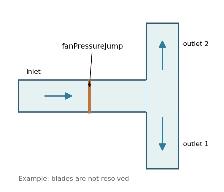
Deep dive · How OpenFOAM 14 applies fanPressureJump, line by line
From the source (fanPressureJumpFvPatchScalarField.C) the condition has two modes:
fanCurve(recommended form): the jump is a function of the total flow rate through the patch, Q = Σ phi (m³/s); the value used is max(f(max(Q, 0)), 0), with the sign reversed ifreverse true.jumpTable(compatibility with the oldfan, used by the tutorial): the jump is a function of the local normal velocity Un = max(phi/|Sf|, 0) face by face, also limited to non-negative values.polynomial (100)is a polynomial with only the zero-degree coefficient: the jump is 100 m²/s² whatever the velocity. Coefficients are written in increasing order of exponent:polynomial (-1 0 1 2)is −1 + x² + 2x³ (Polynomial1.H).- The jump is defined as the value on the neighbour side minus the value on the owner side (fixedJumpFvPatchField.H). Which side is owner depends on the orientation of the
faceZone: in ParaView check that pressure increases across the fan in the flow direction; if it decreases, the flow runs against the zone normal.
To impose an actual ΔP(Q) curve use fanCurve with a table in kinematic units (m³/s; m²/s²), for example derived from the synthetic curve of section 8 divided by the declared density:
p
{
    type            fanPressureJump;
    patchType       cyclic;
    fanCurve        table
    (
        (0      216.7)   // 260 Pa / 1.2 kg/m3
        (0.01   200.0)
        (0.02   170.0)
        (0.03   120.8)
        (0.04    58.3)
    );
    jump            uniform 0;
    value           uniform 0;
}
Beware: the synthetic curve flow rates (up to 0.05 m³/s) are much larger than those possible in a 2 cm duct; for a numerical test in TJunctionFan scale the curve to the order of magnitude of the reference case flow rate. Every change goes into a new copy, not into the guide reference case.
Deep dive · Where the fan is: createZonesDict and the baffle around it
fan
{
    type        surface;
    surface     plate;
    origin      (0.1 -0.006 0.004);
    span        (0 0.012 0.012);
}
baffle
{
    type        difference;
    plane { type plane; point (0.1 0 0); normal (1 0 0); }
    fan;
}
The fan is a 12 × 12 mm square in the x = 0.1 m plane (y from −0.006 to 0.006, z from 0.004 to 0.016), i.e. 9 faces of the 4 mm mesh and 36 % of the 20 × 20 mm duct section. The rest of the same plane (16 faces) is the baffle zone, turned by createBaffles into two walls baffle0/baffle1 with wall functions. All the inlet flow must therefore cross the fan: figure 3 of the guide, which draws the fan over the whole section, is a schematic. With add_monitors.py the flow rate on the fan0 patch is recorded and fan_balance.py checks that it equals the inlet flow.
Practical tip · fanPressure and fanPressureJump: which one to use
fanPressureJump: fan inside the domain, on a pair of cyclic patches created bycreateBaffles; there is fluid upstream and downstream.fanPressure: fan on an inlet or outlet boundary facing the environment: it imposes the ambient total pressurep0plus (inlet) or minus (outlet,direction out) the jump of thefanCurve(v14 documentation).- In both, curves are in the units of the
pfield: kinematic forincompressibleFluid.
7. Exercise B — Internal fan in a T-junction
The second script makes a new, separate copy of the official case:
python3 scripts/prepare_fan_case.py --dest "$HOME/OpenFOAM/guide15_fan_ref"
bash scripts/run_fan_case.sh "$HOME/OpenFOAM/guide15_fan_ref"
The wrapper runs blockMesh, createZones, createBaffles, checkMesh and foamRun in sequence. This preserves the sequence in the Foundation 14 tutorial while adding checkMesh, checks and logs. The exercise deliberately measures the unmodified reference setup rather than inventing an unverified fan curve.
Measure Q in ParaView: create a slice at each opening, calculate the normal component of U, then apply Integrate Variables. With outward normals, check Q_in + Q_out1 + Q_out2 ≈ 0. Integrating U itself as a vector is not the same as volumetric flow unless the normal projection is taken.
Deep dive · Package scripts: prepare_fan_case.py and run_fan_case.sh
prepare_fan_case.py copies the installed tutorial into a new directory (refusing existing ones) and adds GUIDE15_CASE.txt; tested: the comparison with the original shows only that extra file. run_fan_case.sh requires that marker, refuses existing logs and mesh, then runs blockMesh, createZones, createBaffles, checkMesh and foamRun: the tutorial sequence plus checkMesh. Tested with stub commands: a failing foamRun gives exit code 1.
#!/usr/bin/env python3
# SPDX-License-Identifier: GPL-3.0-or-later
"""Safely clone the unmodified OpenFOAM Foundation 14 TJunctionFan tutorial."""
from __future__ import annotations
import argparse
import os
from pathlib import Path
import shutil
import sys


def main() -> int:
    parser = argparse.ArgumentParser(description=__doc__)
    parser.add_argument('--dest', required=True, type=Path)
    args = parser.parse_args()
    root = os.environ.get('FOAM_TUTORIALS')
    if not root:
        parser.error('FOAM_TUTORIALS missing: source the OpenFOAM environment')
    source = Path(root) / 'incompressibleFluid' / 'TJunctionFan'
    if not (source / 'system' / 'createBafflesDict').is_file():
        parser.error(f'Expected tutorial not found: {source}')
    target = args.dest.expanduser().resolve()
    if target.exists():
        parser.error(f'Refusing to overwrite existing directory: {target}')
    target.parent.mkdir(parents=True, exist_ok=True)
    shutil.copytree(source, target)
    (target / 'GUIDE15_CASE.txt').write_text(
        'Reference: OpenFOAM Foundation 14 TJunctionFan\n'
        'Fan pressure jump: unmodified reference tutorial\n'
        'Solver runs: NOT EXECUTED\n', encoding='utf-8')
    print(f'Created {target}')
    return 0


if __name__ == '__main__':
    sys.exit(main())
#!/usr/bin/env bash
# SPDX-License-Identifier: GPL-3.0-or-later
# Run one copy of the Foundation 14 TJunctionFan case without destructive cleanup.
set -euo pipefail
[[ $# -eq 1 ]] || { echo "Usage: bash run_fan_case.sh CASE_DIRECTORY" >&2; exit 2; }
case_dir="$(realpath "$1")"
[[ -f "$case_dir/system/createBafflesDict" && -f "$case_dir/GUIDE15_CASE.txt" ]] || { echo 'Not a prepared Guide 15 fan case' >&2; exit 2; }
cd "$case_dir"
for f in log.blockMesh log.createZones log.createBaffles log.checkMesh log.foamRun; do
[[ ! -e "$f" ]] || { echo "Refusing to overwrite $f" >&2; exit 2; }
done
[[ ! -d constant/polyMesh ]] || { echo 'Existing mesh: refusing to rerun' >&2; exit 2; }
for d in [1-9]*; do
[[ ! -d "$d" ]] || { echo "Existing time directory: $d" >&2; exit 2; }
done
command -v foamRun >/dev/null || { echo 'foamRun not in PATH' >&2; exit 2; }
blockMesh > log.blockMesh 2>&1
createZones > log.createZones 2>&1
createBaffles > log.createBaffles 2>&1
checkMesh > log.checkMesh 2>&1
foamRun > log.foamRun 2>&1
echo "Completed: $case_dir"Technical note: the for d in [1-9]* check does not catch the time directories of this transient case, named 0.1, 0.2, … An already-run case is stopped anyway by the log check that precedes it; if the logs are deleted by hand, that protection is gone. The additional add_monitors.py script recognises any numeric directory other than 0.
Deep dive · Flow balance and split between the outlets (fan_balance.py script)
With the monitors added by add_monitors.py OpenFOAM writes at every step the flow rates on inlet, outlet1, outlet2 and on the fan patch fan0 (postProcessing/Q*/0/surfaceFieldValue.dat). Within the chosen window (by default the last 20 % of the run, hence after the ramp) the script computes means, drift, balance residual, split Qout1/(Qout1 + Qout2) and the ratio of fan to inlet flow (≈ 1 expected), and it can append a row to a CSV with the columns of measurements_template.csv. Tested on synthetic files with a ramp similar to the tutorial one.
C=$HOME/OpenFOAM/guide15_fan_ref; P=$C/postProcessing
python3 add_monitors.py "$C"          # BEFORE run_fan_case.sh
bash scripts/run_fan_case.sh "$C"
python3 fan_balance.py --inlet $P/Qinlet/0/surfaceFieldValue.dat --outlet1 $P/Qoutlet1/0/surfaceFieldValue.dat \
    --outlet2 $P/Qoutlet2/0/surfaceFieldValue.dat --fan $P/Qfan/0/surfaceFieldValue.dat \
    --tstart 1.2 --rho 1.2 --csv measurements.csv
#!/usr/bin/env python3
# SPDX-License-Identifier: GPL-3.0-or-later
"""Flow balance and flow split of the TJunctionFan case (OpenFOAM 14).
Reads the surfaceFieldValue files written by the patchFlowRate monitors of
add_monitors.py (postProcessing/Qinlet/0/surfaceFieldValue.dat, ...; rows:
time and sum(phi) in m3/s, positive when leaving the domain). For a time
window [--tstart, --tend] (default: the last 20 % of the run, after the
inlet total-pressure ramp that ends at t = 1 s in the tutorial) it prints the
mean and the drift of each flow rate, the residual Q_in + Q_out1 + Q_out2
relative to |Q_in|, the split Q_out1/(Q_out1 + Q_out2) and, if given, the
flow through the fan patch as a fraction of the inlet flow.
With --rho the kinematic quantities are converted for a declared density:
mass flow rates [kg/s]. --jump (default 100, the tutorial value) is the
imposed kinematic jump recorded in the CSV. With --csv a NEW row is appended to a measurements
CSV with the columns of resources/measurements_template.csv.
"""
import argparse
import csv
from pathlib import Path
import statistics as st
import sys
def read_sfv(path):
t, q = [], []
with open(path, encoding='utf-8') as f:
for line in f:
s = line.strip()
if not s or s.startswith('#'):
continue
p = s.split()
t.append(float(p[0]))
q.append(float(p[1]))
if not t:
raise ValueError(f'{path}: no data rows')
return t, q
def stats(t, q, t0, t1):
sel = [(a, b) for a, b in zip(t, q) if t0 <= a <= t1]
if len(sel) < 2:
raise ValueError(f'fewer than 2 samples in window {t0}..{t1}')
vals = [b for _, b in sel]
half = len(vals) // 2
drift = st.fmean(vals[half:]) - st.fmean(vals[:half])
return st.fmean(vals), drift, len(vals)
def main():
ap = argparse.ArgumentParser(description=__doc__, formatter_class=argparse.RawDescriptionHelpFormatter)
ap.add_argument('--inlet', type=Path, required=True)
ap.add_argument('--outlet1', type=Path, required=True)
ap.add_argument('--outlet2', type=Path, required=True)
ap.add_argument('--fan', type=Path)
ap.add_argument('--tstart', type=float)
ap.add_argument('--tend', type=float)
ap.add_argument('--rho', type=float, help='declared density [kg/m3] for mass flow rates')
ap.add_argument('--csv', type=Path, help='measurements CSV to append a row to (created if missing)')
ap.add_argument('--case-name', default='guide15_fan_ref')
ap.add_argument('--jump', type=float, default=100.0, help='imposed kinematic fan jump [m2/s2] recorded in the CSV')
a = ap.parse_args()
data = {k: read_sfv(p) for k, p in (('in', a.inlet), ('out1', a.outlet1), ('out2', a.outlet2)) + ((('fan', a.fan),) if a.fan else ())}
tmax = min(v[0][-1] for v in data.values())
t1 = a.tend if a.tend is not None else tmax
t0 = a.tstart if a.tstart is not None else t1 - 0.2 * t1
S = {k: stats(*v, t0, t1) for k, v in data.items()}
print(f'Window t = {t0:g} .. {t1:g} s')
for k, (m, d, n) in S.items():
print(f' Q_{k:5s} = {m: .6g} m3/s (drift between window halves {d: .3g}, {n} samples)')
qin, q1, q2 = S['in'][0], S['out1'][0], S['out2'][0]
res = qin + q1 + q2
print(f'Balance Q_in + Q_out1 + Q_out2 = {res:.3g} m3/s = {100 * res / abs(qin) if qin else float("nan"):.3g} % of |Q_in|')
if q1 + q2:
print(f'Split Q_out1/(Q_out1+Q_out2) = {q1 / (q1 + q2):.4f}')
if 'fan' in S and qin:
print(f'Fan flow / inlet flow = {abs(S["fan"][0]) / abs(qin):.4f} (expected ~1: the rest of the section at x = 0.1 m is a wall baffle, all the inlet flow must cross the fan)')
if a.rho:
print(f'Mass flow rates (rho = {a.rho:g}): in {a.rho * qin:.6g}, out1 {a.rho * q1:.6g}, out2 {a.rho * q2:.6g} kg/s')
if a.csv:
cols = ['case', 'source_tutorial', 'scenario', 'rpm', 'Q_in_m3_s', 'Q_out1_m3_s', 'Q_out2_m3_s',
'delta_p_kinematic_m2_s2', 'rho_kg_m3', 'delta_P_Pa', 'converged', 'mesh_ok', 'notes']
new = not a.csv.exists()
with a.csv.open('a', newline='', encoding='utf-8') as h:
w = csv.writer(h)
if new:
w.writerow(cols)
w.writerow([a.case_name, 'TJunctionFan', f'window {t0:g}-{t1:g} s', '', f'{qin:.8g}', f'{q1:.8g}', f'{q2:.8g}',
f'{a.jump:g}', a.rho or '', (f'{a.jump * a.rho:g}' if a.rho else ''), 'check', 'check',
f'balance {100 * res / abs(qin) if qin else 0:.3g} %'])
print('Row appended to', a.csv)
return 0
if __name__ == '__main__':
try:
sys.exit(main())
except (OSError, ValueError) as exc:
sys.exit(f'ERROR: {exc}')Monitors inserted into the tutorial system/functions (resulting file):
/*--------------------------------*- C++ -*----------------------------------*\
  =========                 |
  \\      /  F ield         | OpenFOAM: The Open Source CFD Toolbox
   \\    /   O peration     | Website:  https://openfoam.org
    \\  /    A nd           | Version:  14
     \\/     M anipulation  |
\*---------------------------------------------------------------------------*/
FoamFile
{
    format      ascii;
    class       dictionary;
    location    "system";
    object      functions;
}
// * * * * * * * * * * * * * * * * * * * * * * * * * * * * * * * * * * * * * //

probes
{
    // Where to load it from
    libs            ("libsampling.so");

    type            probes;

    // Name of the directory for probe data
    name            probes;

    // Write at same frequency as fields
    writeControl    writeTime;
    writeInterval   1;

    // Fields to be probed
    fields          (p U);

    probeLocations
    (
        ( 1e-06 0 0.01 )        // at inlet
        (0.21 -0.20999 0.01)  // at outlet1
        (0.21 0.20999 0.01)   // at outlet2
        (0.21 0 0.01)         // at central block
    );
}

// ---- Guide 15 monitors (added by add_monitors.py) ----
// Volumetric flow rates [m3/s], sum of phi: positive = leaving the domain
#includeFunc patchFlowRate(name=Qinlet, patch=inlet)
#includeFunc patchFlowRate(name=Qoutlet1, patch=outlet1)
#includeFunc patchFlowRate(name=Qoutlet2, patch=outlet2)
// Flow through the fan: sum of phi on the owner side of the cyclic jump
#includeFunc patchFlowRate(name=Qfan, patch=fan0)
// Area-averaged kinematic pressure on the inlet (total pressure BC: p is static)
#includeFunc patchAverage(name=pInlet, patch=inlet, fields=(p))
#includeFunc residuals(p, U, k, epsilon)
// ---- end of Guide 15 monitors ----

// ************************************************************************* //
Practical tip · Flow rate with ParaView without sign ambiguity
- Inlet:
Slicewith origin (0.001, 0, 0.01) and normal (1, 0, 0);Calculatoron cell data with expressionU_X;Integrate Variables: the integral ofU_Xis the incoming flow rate, positive. - Outlets:
Sliceat y = −0.209 and y = +0.209 with normal (0, 1, 0) andCalculatorU_Y. At outlet 1 the flow goes towards −y, so the integral is negative: with outward normals Qout1 = −∫Uy dA and Qout2 = +∫Uy dA. - Check the area returned by
Integrate Variables: it must be 4e-4 m² (20 × 20 mm). A different value indicates a misplaced or badly cut slice. - Choose the same instant (after the ramp) in all cases and write it in the CSV; the comparison with the
fan_balance.pyflow rates is an independent check of the post-processing.
8. Exercise C — Fan and system curves
A credible pressure–flow curve requires multiple operating points, varying system resistance or inlet/outlet conditions in a controlled manner. Record at least rpm (when physically defined), Q, pressure difference, density, case configuration and convergence state. To build a real fan curve with blades, use an appropriate 3D MRF fan geometry; the enclosed mixer case must not be repurposed as a ducted fan.
The kit includes an explicitly synthetic CSV with fan and system curves. plot_fan_curve.py locates intersections using piecewise linear interpolation within the tabulated range and plots the result; it does not extrapolate.

ΔP Q is fluid power, not shaft power or electrical consumption; efficiency needs additional data. Fan affinity relations Q ~ n, ΔP ~ n², P ~ n³ are approximate similarity relationships under comparable flow regimes, not universal laws for the enclosed mixer campaign.
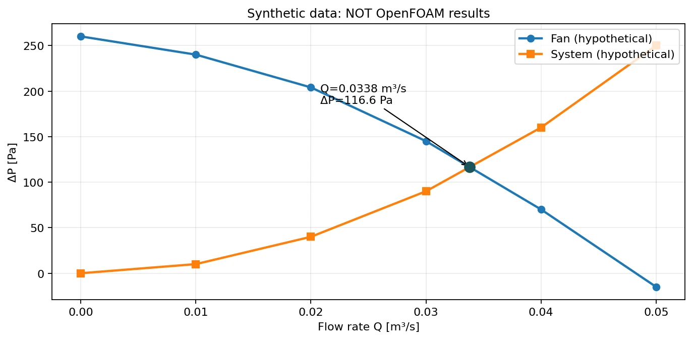
Deep dive · Package script: plot_fan_curve.py, and a corrected defect
The script reads the CSV, checks the columns and that Q is strictly increasing, looks for sign changes of (fan − system) segment by segment and plots without extrapolating. On the synthetic CSV it finds Q = 0.033793 m³/s and ΔP = 116.55 Pa, as in figure 4. Defect: if the intersection falls exactly on a tabulated point it is reported twice, once as the end of the previous segment and once as the start of the next one (tested with a table crossing at Q = 1: two identical output lines). The corrected plot_fan_curve_fixed.py (in the download, extra/ folder) has the same usage and output, but reports each intersection once and also flags equality at the last point when the curves coincide over the last segment.
#!/usr/bin/env python3
# SPDX-License-Identifier: GPL-3.0-or-later
"""Plot fan/system pressure curves from CSV and find bracketed intersections."""
from __future__ import annotations
import argparse
import csv
from pathlib import Path
import sys


def read_rows(filename):
    points = []
    with open(filename, newline='', encoding='utf-8-sig') as file:
        reader = csv.DictReader(file)
        expected = {'Q_m3_s', 'fan_pressure_Pa', 'system_pressure_Pa'}
        if not expected.issubset(set(reader.fieldnames or [])):
            raise ValueError('CSV requires Q_m3_s,fan_pressure_Pa,system_pressure_Pa')
        for row in reader:
            points.append((float(row['Q_m3_s']), float(row['fan_pressure_Pa']), float(row['system_pressure_Pa'])))
    if len(points) < 2 or any(points[i][0] >= points[i+1][0] for i in range(len(points)-1)):
        raise ValueError('At least two rows with strictly increasing Q are required')
    return points


def intersections(points):
    intersections_found = []
    for a, b in zip(points, points[1:]):
        d0 = a[1] - a[2]
        d1 = b[1] - b[2]
        if d0 == 0:
            intersections_found.append((a[0], a[1]))
        if d0 * d1 < 0 or (d0 != 0 and d1 == 0):
            frac = -d0 / (d1 - d0)
            intersections_found.append((a[0] + frac * (b[0] - a[0]), a[1] + frac * (b[1] - a[1])))
    return intersections_found


def main():
    parser = argparse.ArgumentParser(description=__doc__)
    parser.add_argument('--input', required=True, type=Path)
    parser.add_argument('--output', required=True, type=Path)
    parser.add_argument('--allow-overwrite', action='store_true')
    args = parser.parse_args()
    if args.output.exists() and not args.allow_overwrite:
        parser.error('Output exists; choose a new name (or explicitly --allow-overwrite)')
    points = read_rows(args.input)
    hit = intersections(points)
    import matplotlib
    matplotlib.use('Agg')
    import matplotlib.pyplot as plt
    q = [x[0] for x in points]
    fig, ax = plt.subplots(figsize=(7.4, 4.3))
    ax.plot(q, [x[1] for x in points], 'o-', label='Fan curve')
    ax.plot(q, [x[2] for x in points], 's-', label='System curve')
    for qx, px in hit:
        ax.plot([qx], [px], 'ko')
        ax.annotate(f'Q={qx:.5g} m3/s, ΔP={px:.1f} Pa', (qx, px), xytext=(7,9), textcoords='offset points', fontsize=8)
    ax.set(xlabel='Volumetric flow Q [m³/s]', ylabel='Pressure difference [Pa]')
    ax.grid(True, alpha=0.25)
    ax.legend()
    fig.tight_layout()
    fig.savefig(args.output, dpi=160)
    plt.close(fig)
    for qx, px in hit:
        print(f'Intersection in data range: Q={qx:.7g} m3/s, DeltaP={px:.6g} Pa')
    if not hit:
        print('No tabulated-range intersection; no extrapolation performed.')
    return 0


if __name__ == '__main__':
    sys.exit(main())
Complete corrected version, extra/plot_fan_curve_fixed.py (same usage: python3 extra/plot_fan_curve_fixed.py --input resources/fan_system_synthetic.csv --output my_fan_curve.png):
#!/usr/bin/env python3
# SPDX-License-Identifier: GPL-3.0-or-later
"""Plot fan/system pressure curves from CSV and find bracketed intersections.

Guide 15 corrected version of scripts/plot_fan_curve.py: identical usage and
output, but an intersection that coincides with a tabulated point is
reported once instead of twice, and equality at the last tabulated point is
reported also when the curves coincide over the last segment.
"""
from __future__ import annotations
import argparse
import csv
from pathlib import Path
import sys


def read_rows(filename):
    points = []
    with open(filename, newline='', encoding='utf-8-sig') as file:
        reader = csv.DictReader(file)
        expected = {'Q_m3_s', 'fan_pressure_Pa', 'system_pressure_Pa'}
        if not expected.issubset(set(reader.fieldnames or [])):
            raise ValueError('CSV requires Q_m3_s,fan_pressure_Pa,system_pressure_Pa')
        for row in reader:
            points.append((float(row['Q_m3_s']), float(row['fan_pressure_Pa']), float(row['system_pressure_Pa'])))
    if len(points) < 2 or any(points[i][0] >= points[i+1][0] for i in range(len(points)-1)):
        raise ValueError('At least two rows with strictly increasing Q are required')
    return points


def intersections(points):
    intersections_found = []

    def add(q, p):
        # Guide 15 fix: a crossing exactly on a tabulated point was reported
        # twice (end of one segment, start of the next); keep it once.
        if not intersections_found or intersections_found[-1][0] != q:
            intersections_found.append((q, p))

    for a, b in zip(points, points[1:]):
        d0 = a[1] - a[2]
        d1 = b[1] - b[2]
        if d0 == 0:
            add(a[0], a[1])
        if d0 * d1 < 0 or (d0 != 0 and d1 == 0):
            frac = -d0 / (d1 - d0)
            add(a[0] + frac * (b[0] - a[0]), a[1] + frac * (b[1] - a[1]))
    last = points[-1]
    if last[1] - last[2] == 0:
        # Guide 15 fix: equal curves at the last tabulated point (only reached
        # here when the previous segment was already coincident)
        add(last[0], last[1])
    return intersections_found


def main():
    parser = argparse.ArgumentParser(description=__doc__)
    parser.add_argument('--input', required=True, type=Path)
    parser.add_argument('--output', required=True, type=Path)
    parser.add_argument('--allow-overwrite', action='store_true')
    args = parser.parse_args()
    if args.output.exists() and not args.allow_overwrite:
        parser.error('Output exists; choose a new name (or explicitly --allow-overwrite)')
    points = read_rows(args.input)
    hit = intersections(points)
    import matplotlib
    matplotlib.use('Agg')
    import matplotlib.pyplot as plt
    q = [x[0] for x in points]
    fig, ax = plt.subplots(figsize=(7.4, 4.3))
    ax.plot(q, [x[1] for x in points], 'o-', label='Fan curve')
    ax.plot(q, [x[2] for x in points], 's-', label='System curve')
    for qx, px in hit:
        ax.plot([qx], [px], 'ko')
        ax.annotate(f'Q={qx:.5g} m3/s, ΔP={px:.1f} Pa', (qx, px), xytext=(7,9), textcoords='offset points', fontsize=8)
    ax.set(xlabel='Volumetric flow Q [m³/s]', ylabel='Pressure difference [Pa]')
    ax.grid(True, alpha=0.25)
    ax.legend()
    fig.tight_layout()
    fig.savefig(args.output, dpi=160)
    plt.close(fig)
    for qx, px in hit:
        print(f'Intersection in data range: Q={qx:.7g} m3/s, DeltaP={px:.6g} Pa')
    if not hit:
        print('No tabulated-range intersection; no extrapolation performed.')
    return 0


if __name__ == '__main__':
    sys.exit(main())
Deep dive · Operating point with the system parabola and affinity laws (operating_point.py script)
The system values of the synthetic CSV follow exactly ΔP = K Q² with K = 1e5 Pa·s²/m⁶. Linearly interpolating the system curve too, as plot_fan_curve.py does, replaces the parabola with a polyline and moves the operating point: Q = 0.033793 instead of 0.033958 m³/s (−0.5 %) and ΔP = 116.55 instead of 115.32 Pa (+1.1 %). The additional script estimates K by least squares, intersects the fan polyline with the parabola by solving the quadratic in each segment, computes the fluid power and applies the affinity laws: with n2/n1 = 0.8 the point moves along the same parabola with Q × 0.8, ΔP × 0.64 and power × 0.512.
python3 operating_point.py --input resources/fan_system_synthetic.csv --speed-ratio 0.81) Piecewise-linear crossings (as plot_fan_curve.py, without duplicates):
Q = 0.0337931 m3/s, dP = 116.552 Pa
2) System curve fit dP = K Q^2: K = 100000 Pa s2/m6
Q = 0 tabulated 0 fitted 0 residual 0 Pa
Q = 0.01 tabulated 10 fitted 10 residual 0 Pa
Q = 0.02 tabulated 40 fitted 40 residual 0 Pa
Q = 0.03 tabulated 90 fitted 90 residual 0 Pa
Q = 0.04 tabulated 160 fitted 160 residual 0 Pa
Q = 0.05 tabulated 250 fitted 250 residual 0 Pa
3) Fan polyline x fitted parabola:
Q = 0.033958 m3/s, dP = 115.315 Pa -> fluid power dP*Q = 3.916 W
5) Affinity scaling r = n2/n1 = 0.8: fan curve Q x 0.8, dP x 0.64
Q = 0.0271664 m3/s, dP = 73.8015 Pa, fluid power 2.005 W (ratios Q 0.8000, dP 0.6400, power 0.5120)#!/usr/bin/env python3
# SPDX-License-Identifier: GPL-3.0-or-later
"""Fan operating point with a quadratic system curve and affinity scaling.
Input: the CSV of plot_fan_curve.py (Q_m3_s, fan_pressure_Pa,
system_pressure_Pa; strictly increasing Q). The script
1. lists the intersections of the piecewise-linear curves, each one once
(a crossing that falls exactly on a tabulated point is not duplicated);
2. fits the system curve dP = K Q^2 by least squares through the origin,
K = sum(dP Q^2)/sum(Q^4), and reports the residuals;
3. intersects the piecewise-linear fan curve with the fitted parabola,
solving the quadratic exactly in each segment (no extrapolation);
4. prints the fluid power dP*Q at the operating point (not shaft power);
5. with --speed-ratio r it scales the fan curve with the affinity laws
Q2 = r Q1, dP2 = r^2 dP1 (same fan, same density, comparable Reynolds
number) and recomputes the operating point on the same system curve,
showing that a quadratic system moves along Q ~ r, dP ~ r^2.
Theoretical post-processing of tabulated data, not CFD.
"""
import argparse
import csv
import math
from pathlib import Path
import sys
def read_rows(path):
with open(path, newline='', encoding='utf-8-sig') as f:
r = csv.DictReader(f)
need = {'Q_m3_s', 'fan_pressure_Pa', 'system_pressure_Pa'}
if not need.issubset(r.fieldnames or []):
raise ValueError('CSV requires Q_m3_s,fan_pressure_Pa,system_pressure_Pa')
pts = [(float(x['Q_m3_s']), float(x['fan_pressure_Pa']), float(x['system_pressure_Pa'])) for x in r]
if len(pts) < 2 or any(a[0] >= b[0] for a, b in zip(pts, pts[1:])):
raise ValueError('at least two rows with strictly increasing Q are required')
return pts
def linear_crossings(pts):
"""Crossings of fan and system polylines, each reported once."""
out = []
for i, (a, b) in enumerate(zip(pts, pts[1:])):
d0, d1 = a[1] - a[2], b[1] - b[2]
if d0 == 0 and (i == 0 or not out or out[-1][0] != a[0]):
out.append((a[0], a[1]))
if d0 * d1 < 0:
f = -d0 / (d1 - d0)
out.append((a[0] + f * (b[0] - a[0]), a[1] + f * (b[1] - a[1])))
last = pts[-1]
if last[1] - last[2] == 0 and (not out or out[-1][0] != last[0]):
out.append((last[0], last[1]))
return out
def fit_K(pts):
num = sum(p[2] * p[0] ** 2 for p in pts)
den = sum(p[0] ** 4 for p in pts)
if den == 0:
raise ValueError('all Q are zero')
return num / den
def fan_parabola(pts, K, r=1.0):
"""Intersections of the (scaled) piecewise-linear fan curve with dP = K Q^2."""
fan = [(r * q, r * r * f) for q, f, _ in pts]
sols = []
for (q0, f0), (q1, f1) in zip(fan, fan[1:]):
s = (f1 - f0) / (q1 - q0) # f = f0 + s (Q - q0)
A, B, C = K, -s, -(f0 - s * q0) # K Q^2 - s Q - (f0 - s q0) = 0
disc = B * B - 4 * A * C
if disc < 0:
continue
for Q in ((-B + math.sqrt(disc)) / (2 * A), (-B - math.sqrt(disc)) / (2 * A)):
if q0 - 1e-15 <= Q <= q1 + 1e-15 and not any(abs(Q - x) < 1e-12 for x, _ in sols):
sols.append((Q, K * Q * Q))
return sorted(sols)
def main():
ap = argparse.ArgumentParser(description=__doc__, formatter_class=argparse.RawDescriptionHelpFormatter)
ap.add_argument('--input', required=True, type=Path)
ap.add_argument('--speed-ratio', type=float, help='affinity scaling n2/n1 of the fan curve')
a = ap.parse_args()
pts = read_rows(a.input)
print('1) Piecewise-linear crossings (as plot_fan_curve.py, without duplicates):')
for q, p in linear_crossings(pts) or [(None, None)]:
print(' none in the tabulated range' if q is None else f' Q = {q:.6g} m3/s, dP = {p:.6g} Pa')
K = fit_K(pts)
print(f'2) System curve fit dP = K Q^2: K = {K:.6g} Pa s2/m6')
for q, _, s in pts:
print(f' Q = {q:<8g} tabulated {s:<8g} fitted {K * q * q:<10.4g} residual {s - K * q * q:.3g} Pa')
print('3) Fan polyline x fitted parabola:')
op = fan_parabola(pts, K)
for q, p in op or [(None, None)]:
if q is None:
print(' none in the tabulated range')
else:
print(f' Q = {q:.6g} m3/s, dP = {p:.6g} Pa -> fluid power dP*Q = {p * q:.4g} W')
if a.speed_ratio:
r = a.speed_ratio
print(f'5) Affinity scaling r = n2/n1 = {r:g}: fan curve Q x {r:g}, dP x {r * r:g}')
for q, p in fan_parabola(pts, K, r) or [(None, None)]:
if q is None:
print(' no intersection inside the scaled tabulated range (no extrapolation)')
else:
msg = f' Q = {q:.6g} m3/s, dP = {p:.6g} Pa, fluid power {p * q:.4g} W'
if op:
msg += f' (ratios Q {q / op[0][0]:.4f}, dP {p / op[0][1]:.4f}, power {p * q / (op[0][0] * op[0][1]):.4f})'
print(msg)
return 0
if __name__ == '__main__':
try:
sys.exit(main())
except (OSError, ValueError) as exc:
sys.exit(f'ERROR: {exc}')Deep dive · Package example files
fan_system_synthetic.csv is explicitly synthetic (it does not come from OpenFOAM); measurements_template.csv only contains the header of the columns to fill in for each case. The package plot fan_system_demo.png is the output of plot_fan_curve.py on that CSV.
Q_m3_s,fan_pressure_Pa,system_pressure_Pa
0.000,260,0
0.010,240,10
0.020,204,40
0.030,145,90
0.040,70,160
0.050,-15,250
case,source_tutorial,scenario,rpm,Q_in_m3_s,Q_out1_m3_s,Q_out2_m3_s,delta_p_kinematic_m2_s2,rho_kg_m3,delta_P_Pa,converged,mesh_ok,notes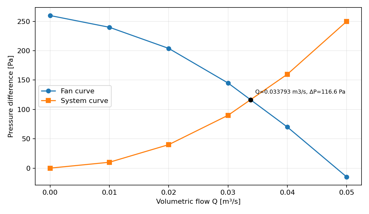
Package resources/fan_system_demo.png: synthetic data, not OpenFOAM results.
Practical tip · How to actually obtain a system or fan curve with OpenFOAM
- System curve: replace the fan with a known jump (for example
jumpTable polynomial (0)and several constant inlet total pressures) and record the (Q, Δp) pair for each copy; the ratio Δp/Q² tells whether the system is quadratic in the explored range. - Operating point with an imposed curve: tabulated
fanCurve(section 6): the solver finds by itself the intersection between the imposed curve and the resistance of the domain. - Fan curve from geometry: 3-D impeller with MRF (like
simpleRushtonMRFfor mixers) or moving mesh, one simulation for each imposed outlet pressure; for each point: Q, total-pressure rise, torque and hence efficiency ΔPt Q/(M ω). - For reference experimental fan testing: ISO 5801:2017, “Fans — Performance testing using standardized airways” (standard record).
Deep dive · Affinity laws: where they come from and when they stop holding
For geometrically similar machines, dimensional analysis links the flow coefficient φ = Q/(N D³), the pressure coefficient ψ = ΔP/(ρ N² D²) and the power coefficient P/(ρ N³ D⁵) to the Reynolds number and the relative roughness. If Re is high enough to make its influence negligible (fully turbulent regime) and the fluid is incompressible, at equal φ the values of ψ and efficiency stay constant: hence Q ∝ N, ΔP ∝ N², P ∝ N³ for the same machine. The laws lose validity at low Re (exactly the case of this guide’s MRF campaign), when the duty point changes (non-quadratic systems, for example with a static pressure to overcome) and with compressibility or cavitation effects. Classic reference: S. L. Dixon, C. A. Hall, Fluid Mechanics and Thermodynamics of Turbomachinery, 7th ed., Butterworth-Heinemann 2014, ch. 1–2.
9. Quantitative ParaView post-processing on Windows
Run pvserver on Linux and connect ParaView 5.13.2 from Windows through the SSH tunnel discussed in Guide 1. Load the OpenFOAM case and save a separate .pvsm state for each setup. Use consistent color scales for meaningful comparisons.
Recommended operations:
Slicethrough the rotation axis or device; color bymag(U).Stream Tracerwith reproducible seed locations, remembering that MRF outputs mean fields.Plot Over LineandProbe Locationfor quantitative profiles.Calculatorfor normal U followed byIntegrate Variableson the flow section to obtain Q.Save Datafor CSV andSave Statefor reproducible.pvsmsessions.
For pressure, convert kinematic pressure to Pa with a documented density and distinguish static, total and imposed fan pressure changes.
Practical tip · Relative velocity and cylindrical components in ParaView
- In the MRF case
Uis the absolute velocity. To see the flow as the impeller sees it, in the rotor zone only:Calculatoron cell data withU - (-6.2832*coordsY)*iHat - (6.2832*coordsX)*jHat(ω = 6.2832 rad/s at 60 rpm, z axis). Streamlines of the relative velocity in the rotor and of the absolute velocity in the stator are the two pictures that make sense in an MRF field. - Radial and tangential components: the OpenFOAM
cylindricalfunction (used by themixerVessel2Dtutorial) writescylindrical(U)for a given origin and axis; in ParaView the same is obtained with aCalculator(Uθ = (x Uy − y Ux)/r). - In the 2-D case use the
Sliceat z = 0 or the cell data directly: the depth is a single cell.
# OpenFOAM alternative, after the run, in the case directory
foamPostProcess -func "cylindrical(field=U, origin=(0 0 0), axis=(0 0 1))" -latestTime
10. Convergence, conservation and validation
Residual stabilization alone is not physical validation. Report mass conservation across measurement sections, mesh independence, rpm and stability of integrated observables. In MRF, inspect how near-impeller flow changes with grid resolution. In the internal fan case, verify fan surface position and pressure-jump sign.
Optional refresher. Real machines may involve cavitation, compressibility, turbulence, rotor–stator interaction and three-dimensional blade geometry. The 2D MRF mixer teaches the numerical method; it does not certify a commercial fan.
Deep dive · Concrete numerical verification plan for the MRF campaign
- Convergence: initial residuals, rotor torque stable within 0.1 % over the last 50 iterations and balance Mz,rotor + Mz,stator within 1 % (
mrf_torque.py); if needed, continue beyond 500 iterations in a copy. - Mesh: copy the shared dictionary into
system/blockMeshDictand doublenCellsRootTip,nCellsMidandnCellsBladeBlade(12 → 24, 4 → 8, 12 → 24): 12,288 cells. Sincerun_mrf_case.shalways uses the official dictionary, run the commands by hand in the fine copy. With three levels apply the GCI of Guide 4 to the torque. - Model: laminar versus k-ε (section 5).
- Method: comparison with the moving mesh (next box).
cp "$FOAM_TUTORIALS/resources/blockMesh/mixerVessel2D" system/blockMeshDict
foamDictionary system/blockMeshDict -entry nCellsRootTip -set 24
foamDictionary system/blockMeshDict -entry nCellsMid -set 8
foamDictionary system/blockMeshDict -entry nCellsBladeBlade -set 24
blockMesh > log.blockMesh 2>&1 && checkMesh > log.checkMesh 2>&1 && foamRun > log.foamRun 2>&1
Deep dive · Comparison with the moving mesh: mixerVessel2D, same geometry
The mixerVessel2D tutorial uses the same mesh dictionary, separates rotor and stator on the r = 0.06 m cylinder with createBaffles and splitBaffles, couples them with createNonConformalCouples and turns the rotor with a solidBody rotatingMotion at omega 60 [rpm] for 5 s (5 revolutions, maxCo 0.5). Before comparing it with MRF three differences present in the tutorials must be aligned:
- model:
laminarversus k-ε; - rotor walls:
movingWallSlipVelocity(slip) versusMRFnoSlip(no slip); - time: the moving case is transient and must be averaged over an integer number of revolutions after the initial transient (its
system/functionsalready averages the cylindrical componentscylindrical(U)).
Then compare the mean Uθ profiles along the same radius and the mean torque: the difference measures the “frozen rotor” error for this geometry.
# moving-mesh tutorial, Allrun
blockMesh -dict $FOAM_TUTORIALS/resources/blockMesh/mixerVessel2D
createBaffles
splitBaffles
createNonConformalCouples nonCouple1 nonCouple2
foamRun
11. Common problems
| Symptom | First check |
|---|---|
rotor cellZone missing | Wrong mesh dictionary; check blockMesh and constant/polyMesh/cellZones |
| All rpm cases look identical | Inspect MRFProperties, actual run directories and loaded time |
createBaffles fails | Verify prior createZones, matching face-zone names and no repeated operations |
| Flow balance fails | Check section normals, section placement and numerical convergence |
p labelled Pa | Inspect dimensions: [kinematicPressure] means m²/s² |
| No curve intersection | Ranges may not overlap; never fabricate an extrapolated operating point |
Practical tip · Actual error messages and what they mean
| Message | Cause and remedy |
|---|---|
Walls rotating in the MRF region should have the MRFnoSlip boundary condition | no U patch has an MRF condition: rotor set to noSlip |
Rotational speeds rpm and omega both defined | MRFProperties contains both rpm and omega |
Neither rotational speed rpm nor omega defined | speed missing or written with a different keyword |
rotor zone not found | mesh generated without the shared dictionary: the blocks named rotor create the cellZone |
dimensions of phi are not correct | fanPressureJump on a case whose flux has unexpected dimensions (neither volumetric nor mass) |
negative branch-1 flow rates in patchFlowRate | backflow from the p = 10 m²/s² outlet: possible at the start of the ramp; inletOutlet handles it, but it must be reported |
12. Windows–Linux workflow and data safety
Keep Windows as the working environment for Notepad++, FileZilla SFTP and ParaView client-server. Use PowerShell/SSH for Linux commands and batch launching only. Separate case inputs, outputs, logs and CSV; never automatically delete completed simulations or overwrite data.
Suggested structure: guide15_MRF/mrf_0030rpm, mrf_0060rpm, mrf_0120rpm, and guide15_fan_ref. Keep data-provenance CSV records and manual-change notes.
Practical tip · Reproducible archive of a campaign
Once the run is finished, archive inputs, logs, postProcessing and CSV together, with checksums, without touching the original cases:
cd "$HOME/OpenFOAM"
foamVersion > guide15_versions.txt
tar czf guide15_archive_$(date +%Y%m%d).tar.gz guide15_MRF guide15_fan_ref guide15_versions.txt \
    --exclude="processor*"
sha256sum guide15_archive_*.tar.gz > guide15_archive.sha256
13. Scientific hand-off checklist
- ☐ OpenFOAM Foundation 14 release, reference tutorial and parameters recorded.
- ☐ Mesh, MRF cell zone or fan baffle checked; logs retained.
- ☐ rpm, viscosity, density and dimensions documented.
- ☐ Residuals, flow balances and integral observables reviewed.
- ☐ Measurement surfaces and normals specified.
- ☐ Plots and CSV based on actual CFD data or clearly labelled synthetic.
- ☐
.pvsm, scripts, case files and results archived without overwrites.
Practical tip · Additional items for a research hand-off
- Declared density and its rationale (air, liquid) written next to every value in Pa.
- For MRF: torque, angular-momentum balance, power and Np‘ for each speed; interface position and “frozen rotor” limitation stated.
- For the fan case: time window of the measurements, flow balance, split between outlets, jump direction verified.
- Turbulence model justified against the Reynolds number, or comparison with the laminar run.
- Additional scripts used and their version (SHA-256 sums in the
README_IT_EN.txtof the download).
14. Official references
- Foundation 14
mixerVessel2DMRFtutorial: https://github.com/OpenFOAM/OpenFOAM-14/tree/master/tutorials/incompressibleFluid/mixerVessel2DMRF - Foundation 14
TJunctionFantutorial: https://github.com/OpenFOAM/OpenFOAM-14/tree/master/tutorials/incompressibleFluid/TJunctionFan - Foundation 14
MRFProperties: https://github.com/OpenFOAM/OpenFOAM-14/blob/master/tutorials/incompressibleFluid/mixerVessel2DMRF/constant/MRFProperties - Foundation 14 internal fan baffle setup: https://github.com/OpenFOAM/OpenFOAM-14/blob/master/tutorials/incompressibleFluid/TJunctionFan/system/createBafflesDict
- Foundation 14
fanPressureAPI: https://cpp.openfoam.org/v14/classFoam_1_1fanPressureFvPatchScalarField.html
New exercise scripts and illustrative figures: GNU GPL v3 or later. Original tutorial cases retain their own licences and are not bundled as copies.
Deep dive · Reference reading, with links
- J. Y. Luo, R. I. Issa, A. D. Gosman, «Prediction of impeller-induced flows in mixing vessels using multiple frames of reference», IChemE Symposium Series 136 (1994) 549–556.
- A. Brucato, M. Ciofalo, F. Grisafi, G. Micale, «Numerical prediction of flow fields in baffled stirred vessels: a comparison of alternative modelling approaches», Chem. Eng. Sci. 53 (1998) 3653–3684, doi:10.1016/S0009-2509(98)00149-3.
- J. H. Rushton, E. W. Costich, H. J. Everett, «Power characteristics of mixing impellers», Chem. Eng. Prog. 46 (1950) 395–404 e 467–476.
- E. L. Paul, V. A. Atiemo-Obeng, S. M. Kresta (eds.), Handbook of Industrial Mixing: Science and Practice, Wiley 2004.
- B. E. Launder, D. B. Spalding, «The numerical computation of turbulent flows», Comput. Methods Appl. Mech. Eng. 3 (1974) 269–289, doi:10.1016/0045-7825(74)90029-2.
- S. L. Dixon, C. A. Hall, Fluid Mechanics and Thermodynamics of Turbomachinery, 7th ed., Butterworth-Heinemann 2014.
- ISO 5801:2017, Fans — Performance testing using standardized airways, standard record.
- CFD Direct, Non-Conformal Coupling (non-conformal interfaces in OpenFOAM Foundation).
Deep dive · The OpenFOAM 14 source files cited in the boxes
- MRFZone.C / MRFZones.C — Coriolis, relative fluxes, zone faces
- MRFnoSlipFvPatchVectorField.C — rotating wall
- omega1.H — omega, rpm and units
- fanPressureJumpFvPatchScalarField.H / .C — fanCurve and jumpTable
- fanPressureFvPatchScalarField.C — fan on a boundary
- fixedJumpFvPatchField.H — jump definition
- forcesBase.C — forces.dat format
- forcesIncompressible, patchFlowRate, power — functions used by the monitors
Deep dive · Package files and additional scripts of this article
| File | Where it is reproduced | Status |
|---|---|---|
scripts/prepare_mrf_cases.py | section 5 | from the package, tested on the tutorial |
scripts/run_mrf_case.sh | section 5 | from the package, tested with stubs |
scripts/prepare_fan_case.py | section 7 | from the package, tested on the tutorial |
scripts/run_fan_case.sh | section 7 | from the package, tested with stubs |
scripts/plot_fan_curve.py | section 8 | from the package, intersection defect documented |
resources/*.csv | section 8 | from the package (synthetic / template) |
plot_fan_curve_fixed.py | section 8 | additional, fix, tested |
operating_point.py | section 8 | additional, tested |
add_monitors.py | section 5 | additional, tested on real copies |
mrf_torque.py | section 5 | additional, tested on synthetic files |
mrf_scaling.py | section 5 | additional, tested on synthetic profiles |
fan_balance.py | section 7 | additional, tested on synthetic files |
g15_estimates.py | section 3 | additional, tested |
Related guides: Linux server from Windows, monitoring and convergence, ParaView for quantitative analysis, verification and validation, parameter sweeps, mesh generation and quality checks, boundary conditions and physical models, transient simulations, turbulence and RANS models, heat transfer and natural convection, conjugate heat transfer, species transport, diffusion and mixing, multiphase flows and VOF interfaces, porous media and pressure loss and the Learning OpenFOAM 14 path.
Download: scripts and files of the guide
The archive OpenFOAM14_Guida15_script.zip (100 kB compressed, 17 files) contains every script and data file reproduced or cited in this article, with the same content as the boxes: the scripts/, examples/ and similar folders hold the guide package files, extra/ the additional scripts and files presented in the deep dives. README_IT_EN.txt lists the contents with SHA-256 checksums; files marked SYNTHETIC are illustrative data, not CFD results. Licence GNU GPL v3 or later (COPYING_GPLv3.txt).
Important: to record torque, power and flow rates run python3 extra/add_monitors.py on every new copy before run_mrf_case.sh or run_fan_case.sh (sections 5 and 7); for the plot use extra/plot_fan_curve_fixed.py, which fixes the duplicate intersections (section 8); in the fan case measure after the pressure ramp that ends at t = 1 s.
Archive contents:
extra/add_monitors.py— Add Guide 15 monitoring function objects to a NEW, not yet run, case copy.extra/fan_balance.py— Flow balance and flow split of the TJunctionFan case (OpenFOAM 14).extra/functions_guide15_fan_example— example TJunctionFan system/functions after add_monitors.py (tutorial probes + Guide 15 monitors)extra/functions_guide15_mrf_example— example system/functions generated by add_monitors.py for an MRF case (rhoInf 1000)extra/g15_estimates.py— Order-of-magnitude checks for the two Guide 15 tutorials (OpenFOAM 14).extra/mrf_scaling.py— Similarity check of the MRF campaign from ParaView Plot Over Line exports.extra/mrf_torque.py— Torque, power and torque balance of an MRF mixer from OpenFOAM 14 forces files.extra/operating_point.py— Fan operating point with a quadratic system curve and affinity scaling.extra/plot_fan_curve_fixed.py— corrected scripts/plot_fan_curve.py: same usage and output, each intersection reported onceresources/fan_system_demo.png— plot produced by plot_fan_curve.py on the SYNTHETIC CSV (not CFD results)resources/fan_system_synthetic.csv— SYNTHETIC / illustrative data, not CFD results (7 lines)resources/measurements_template.csv— CSV data or template (1 lines)scripts/plot_fan_curve.py— Plot fan/system pressure curves from CSV and find bracketed intersections.scripts/prepare_fan_case.py— Safely clone the unmodified OpenFOAM Foundation 14 TJunctionFan tutorial.scripts/prepare_mrf_cases.py— Create non-overwriting OpenFOAM 14 MRF training cases from the installed tutorial.scripts/run_fan_case.sh— Run one copy of the Foundation 14 TJunctionFan case without destructive cleanup.scripts/run_mrf_case.sh— Run one prepared MRF case. Existing results and logs are never overwritten.