OpenFOAM 14 Case 02: Mesh Convergence Study on a Laminar Channel

22 September 2026 by giux CFD and OpenFOAM 7 min read

In Case 01 the parallel-plate channel reproduces the Poiseuille profile with a 0.15% error. One question remains: does that result depend on the chosen mesh? This second case of the Learning OpenFOAM 14 path isolates the effect of spatial discretization. Below is the complete report of the simulation, section by section.

CFD Simulation 02 – Mesh Convergence Study
Laminar channel flow between parallel plates
OpenFOAM Foundation 14 | ParaView 5.13.2 | steady incompressible flow

1. Purpose and result

Simulation 02 isolates the numerical effect of spatial discretization. The physical model, boundary conditions, solver, numerical schemes and post-processing procedure are kept unchanged from the validated laminar-channel benchmark. Only the mesh density is varied.

Key result
The normalized RMSE decreases from 0.528373% to 0.132544% to 0.034843% as the mesh is refined. The observed convergence order from coarse to medium is 1.995 and from medium to fine is 1.928, which is consistent with approximately second-order grid convergence for this smooth benchmark.

Acceptance criteria

All three meshes pass checkMesh.
The three cases use identical physics and boundary conditions.
The velocity profile converges monotonically toward the analytical Poiseuille solution.
The error decreases systematically under a factor-two refinement of the cell size.
The visual flow topology remains unchanged, as expected for the same physical problem.

Measured results

Mesh	Cells	U_max [m/s]	NRMSE [%]	Max error [%]
Coarse	2,000	0.014925373	0.528373	0.744973
Medium	8,000	0.014981273	0.132544	0.185344
Fine	32,000	0.014993729	0.034843	0.056936

2. Physical and numerical baseline

The benchmark is the same steady laminar channel used in Simulation 01. The purpose of reusing the same case is to eliminate changes in physics while evaluating mesh dependence.

Parameter	Value
Geometry	Length 0.500 m; gap 0.010 m; numerical depth 0.001 m
Fluid	Water-like incompressible fluid, kinematic viscosity nu = 1e-6 m²/s
Mean inlet velocity	0.010 m/s
Flow regime	Laminar; Reynolds number based on hydraulic diameter approximately 200
Solver	`foamRun` with solver `incompressibleFluid`
Time treatment	`steadyState`
Analytical reference	Plane Poiseuille flow
Analytical U_max	0.015000000 m/s
Profile sampling	x = 0.45 m across y, 201 uniformly spaced points

What is intentionally unchanged

Geometry and dimensions
Inlet, outlet and wall boundary conditions
Fluid properties
Momentum transport model
fvSchemes and fvSolution
Steady stopping criterion and output cadence
Sampling location and analytical reference

What changes

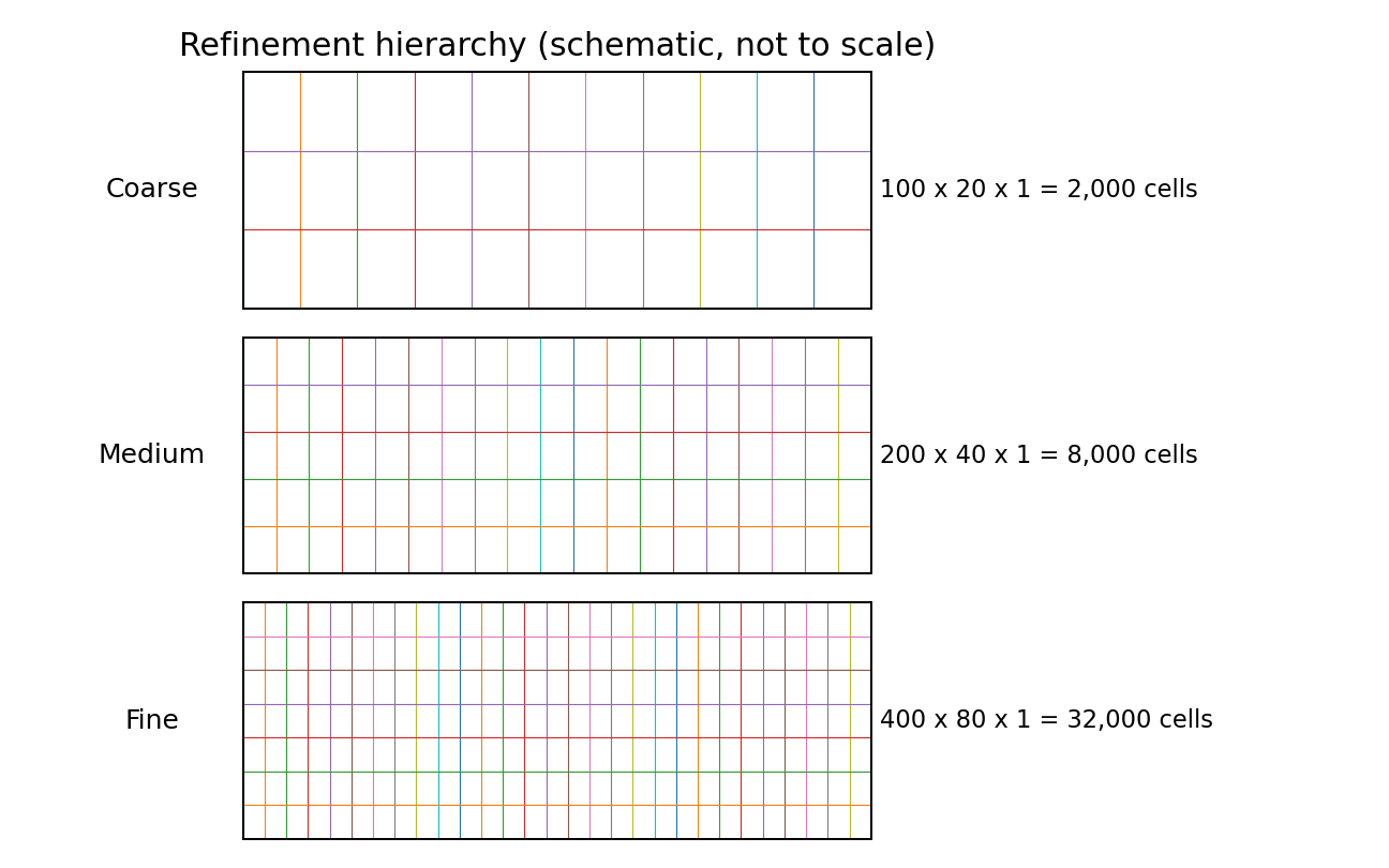
Only the blockMesh cell counts are changed. N_x and N_y are refined together so that the cell aspect ratio is preserved and the characteristic cell size is approximately halved at each level.

Refinement hierarchy with 2,000, 8,000 and 32,000-cell meshes — Refinement hierarchy (schematic, not to scale): coarse 100 x 20 x 1 = 2,000 cells; medium 200 x 40 x 1 = 8,000 cells; fine 400 x 80 x 1 = 32,000 cells.

3. Case preparation

Starting from the validated Simulation 01 setup, three independent cases are created under 02_mesh_convergence. The initial fields, material properties and system dictionaries are copied unchanged.

cd $FOAM_RUN
mkdir -p 02_mesh_convergence/{coarse,medium,fine}

for c in coarse medium fine; do
    cp -a 01_laminar_channel/0         02_mesh_convergence/$c/
    cp -a 01_laminar_channel/constant  02_mesh_convergence/$c/
    cp -a 01_laminar_channel/system    02_mesh_convergence/$c/
done

Mesh definitions

# Coarse
sed -i 's/(200 40 1)/(100 20 1)/' 02_mesh_convergence/coarse/system/blockMeshDict

# Medium remains unchanged
# (200 40 1)

# Fine
sed -i 's/(200 40 1)/(400 80 1)/' 02_mesh_convergence/fine/system/blockMeshDict

Mesh generation and quality check

for c in coarse medium fine; do
    echo "===== $c ====="
    cd $FOAM_RUN/02_mesh_convergence/$c
    blockMesh > log.blockMesh
    checkMesh > log.checkMesh
    grep -E "cells:|max aspect ratio|Max aspect ratio|Mesh OK" log.checkMesh
done

Expected cell counts are 2,000, 8,000 and 32,000. All meshes were reported as acceptable by checkMesh before solving.

4. Uniform post-processing definition

Each case is sampled at the same physical location and with the same 201-point line. This avoids changing the comparison grid together with the CFD grid and ensures that y = 0 is included explicitly.

FoamFile
{
    format          ascii;
    class           dictionary;
    object          graphUniform;
}

start           (0.45 -0.0049 0.0005);
end             (0.45  0.0049 0.0005);
nPoints         201;
fields          (U);
axis            y;

#includeEtc "caseDicts/postProcessing/graphs/graphUniform.cfg"

Execution

cd $FOAM_RUN/02_mesh_convergence

for c in coarse medium fine; do
    cd $FOAM_RUN/02_mesh_convergence/$c
    foamRun | tee log.foamRun
    foamPostProcess -solver incompressibleFluid -func graphUniform -latestTime
done

The three cases therefore differ only in their spatial discretization. The solver and post-processing path are identical.

5. Quantitative convergence results

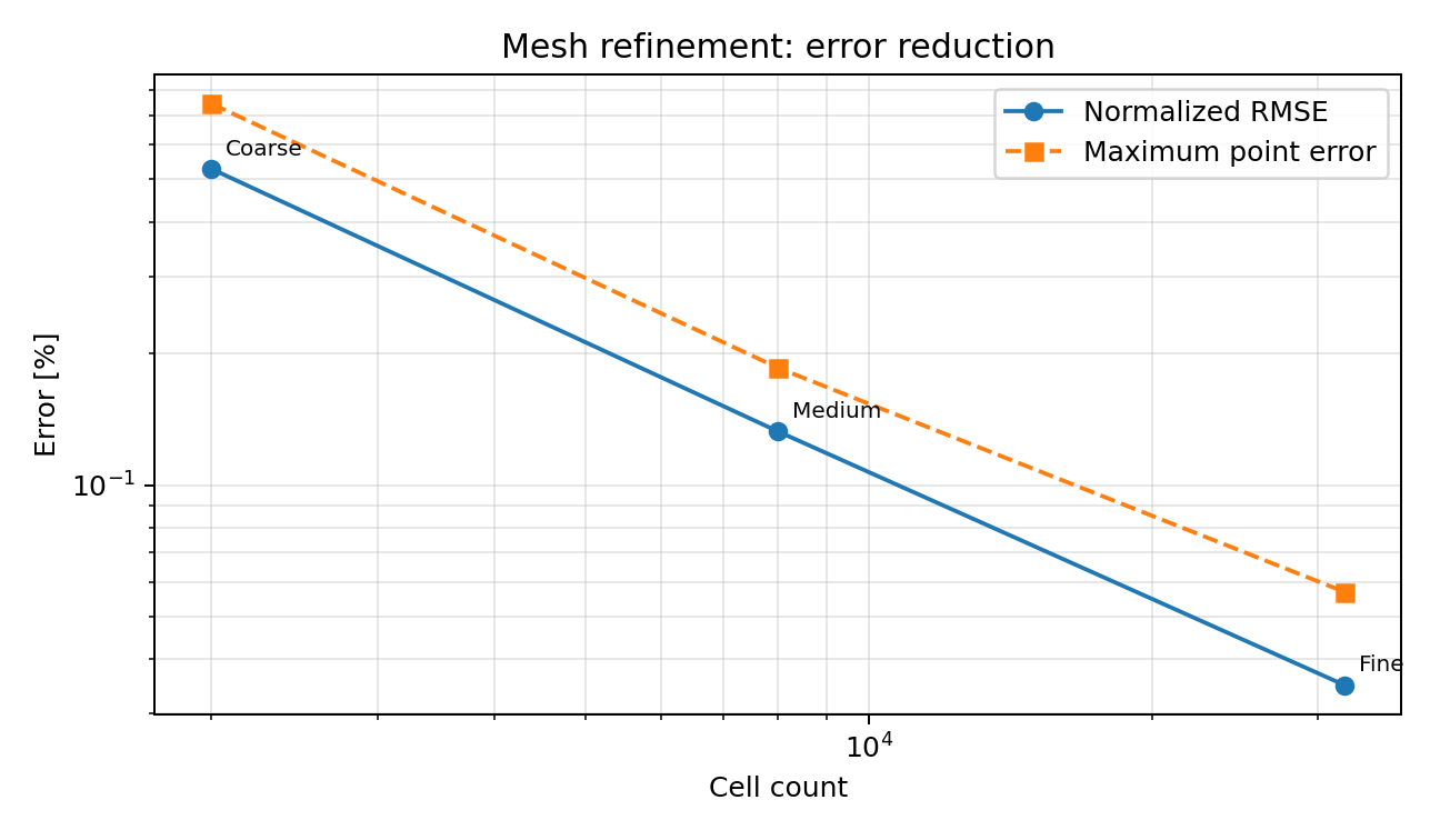
Normalized error versus cell count in the mesh convergence study — Mesh refinement: error reduction (normalized RMSE and maximum point error versus cell count).

Both global and pointwise error measures decrease monotonically with refinement. The normalized RMSE is the principal metric because it represents the error over the complete sampled velocity profile rather than one isolated location.

Observed convergence order

For a refinement ratio r = 2, the observed order p is estimated from p = log(E₁/E₂) / log(r). Using normalized RMSE:

coarse -> medium:
p = log(0.528373 / 0.132544) / log(2) = 1.995

medium -> fine:
p = log(0.132544 / 0.034843) / log(2) = 1.928

Interpretation
The error reduction is close to the factor of four expected from a second-order method when the characteristic mesh spacing is halved. The benchmark therefore shows approximately second-order grid convergence over the tested refinement range.

Maximum pointwise error

The maximum pointwise error also decreases monotonically: 0.744973%, 0.185344%, and 0.056936%. Its medium-to-fine convergence is less regular than the profile-wide RMSE because a maximum metric is more sensitive to interpolation and the exact sample location.

6. Convergence of maximum velocity

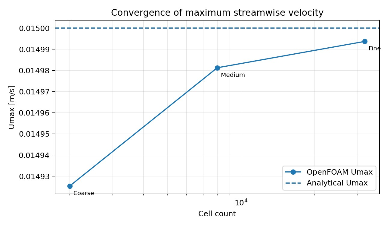
Computed maximum velocity converging to the analytical 0.015 m/s — Convergence of maximum streamwise velocity: OpenFOAM U_max versus analytical U_max.

For plane Poiseuille flow with mean velocity 0.010 m/s, the analytical centerline velocity is U_max = 1.5 U_mean = 0.015 m/s. The computed values approach this limit monotonically.

Mesh	U_max [m/s]	Relative U_max error [%]	Trend
Coarse	0.014925373	0.497513	Toward 0.015 m/s
Medium	0.014981273	0.124847	Toward 0.015 m/s
Fine	0.014993729	0.041807	Toward 0.015 m/s

The coarse-to-medium U_max error ratio is consistent with approximately second-order behavior. At the finest grid the absolute error is already very small, so interpolation and sampling effects become more visible in derived order estimates.

7. ParaView verification

All three result sets were opened concurrently through the existing ParaView client-server session. The Windows client remained connected to pvserver; only the pipeline objects were changed.

Remote case markers

cd $FOAM_RUN/02_mesh_convergence
touch coarse/coarse.foam
touch medium/medium.foam
touch fine/fine.foam

The three .foam markers allow ParaView to open each case directly from the remote Linux filesystem.

Recommended display configuration

Select one case at a time when inspecting cell density, because the external geometry is identical and the three datasets otherwise overlap.
Use Representation = Surface With Edges for direct mesh inspection.
Use Representation = Outline when the goal is to keep the domain reference visible without obscuring streamlines.
Keep internalMesh enabled with U and p loaded; individual boundary patches are not required for the general field view.

Streamline check

The streamline calculation is not a new CFD solution. It is a post-processing integration through the steady U field. The same seed definition used in Simulation 01 is sufficient:

Vectors                   = U
Integration Direction     = FORWARD
Seed Type                 = Line
Point1                    = (0.001, -0.0045, 0.0005)
Point2                    = (0.001,  0.0045, 0.0005)
Resolution                = 20
Maximum Streamline Length = 0.5

The streamline topology is essentially identical for coarse, medium and fine meshes: straight, parallel paths in the streamwise direction. This is the expected result because the underlying physical problem has not changed. The meaningful mesh-dependence is in the numerical accuracy of the velocity field, not in a change of flow topology.

8. Interpretation and engineering use

What this study establishes

The solution is not an artifact of one particular grid.
The computed profile converges systematically toward the analytical solution.
The observed error reduction is consistent with approximately second-order behavior.
For this benchmark, 8,000 cells already give NRMSE about 0.13%, while 32,000 cells reduce it to about 0.035%.
Further refinement of this simple benchmark would mainly have didactic value rather than changing the engineering conclusion.

What this study does not establish

It does not prove that 8,000 or 32,000 cells are sufficient for the future reactor geometry.
It does not transfer a cell count from this simple channel to a complex reactor.
It does not eliminate the need for a reactor-specific mesh-independence study, especially around inlets, recirculation regions and porous-grid representations.

Practical consequence
The workflow is now validated: define a refinement family, keep the physics fixed, sample the same observables, compute numerical error, estimate convergence order, then inspect the result visually. The same methodology can later be applied to the reactor with a suitable reference quantity even when no analytical solution exists.

9. Reproduction checklist

Start from the validated 01_laminar_channel case.
Create coarse, medium and fine copies.
Set block counts to 100 x 20 x 1, 200 x 40 x 1, and 400 x 80 x 1.
Run blockMesh and checkMesh for each case.
Use the same physicalProperties, momentumTransport, fvSchemes, fvSolution, U and p definitions.
Run foamRun to the established steady endpoint.
Post-process U at x = 0.45 m with 201 common sample points.
Compare every sample against the analytical Poiseuille profile.
Calculate NRMSE and maximum absolute error normalized to analytical U_max.
Estimate observed order using r = 2.
Open the three .foam markers through pvserver and compare mesh density and field behavior.
Use Outline plus Stream Tracer when a clean trajectory view is required.

Final status
SIMULATION 02 – COMPLETE
Coarse, medium and fine meshes were solved successfully. Velocity-profile error decreases monotonically with refinement, the observed profile-wide convergence order is approximately two, and ParaView verification confirms unchanged laminar flow topology across all three grids.

In Case 03 the same channel is rebuilt with a Gmsh mesh instead of blockMesh.

#CFD #CFD validation #mesh #OpenFOAM #Poiseuille flow