

OpenFOAM 14 Part 7: Physical Properties and Models
This is Part 7 of the case-construction series of the Learning OpenFOAM 14 project. After the solution and algorithm controls of Part 6 (fvSolution), we move from how the equations are solved to which equations are solved: fluid properties in constant/physicalProperties and models of momentum transport in constant/momentumTransport.
The thread of the whole part is a single chain: a fluid datum (nu) feeds a stress model, and the stress model decides which fields must exist in 0/. Changing a number is a change of material; changing a model is a change of mathematics, with consequences across the whole case. Everything is for OpenFOAM Foundation 14 (openfoam.org / CFD Direct), single-phase incompressible reference channel.
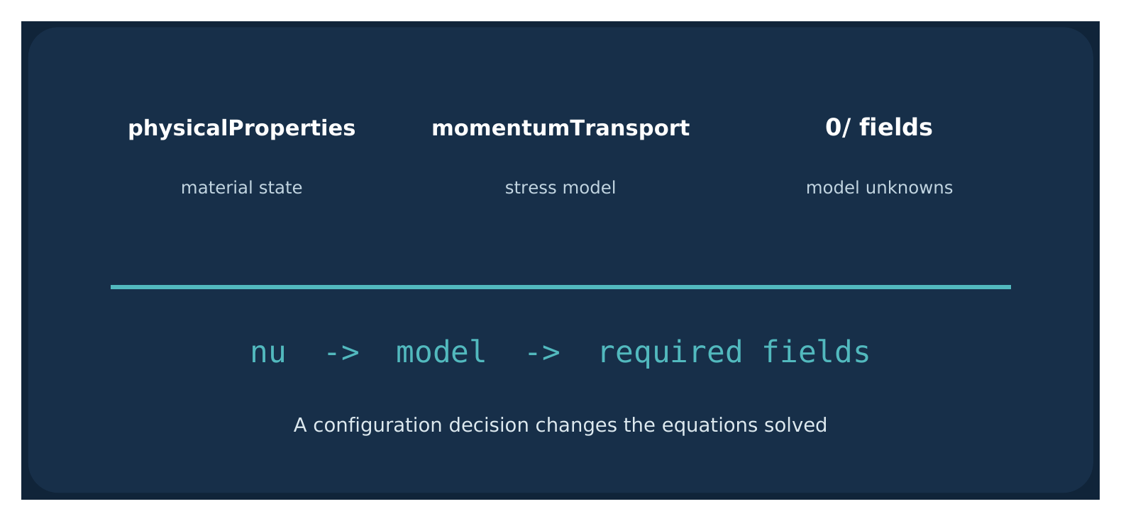
Prerequisites: the initial CFD exercises of the project (starting from the laminar channel / Poiseuille case) and Parts 1–6. Scope: OpenFOAM Foundation 14, single-phase incompressible reference channel. Method: concept → dictionary → model consequences → experiment.
Before you begin
This part teaches the difference between fluid properties and models of momentum transport. It reuses the same basic incompressible channel as the previous units; do not modify the teaching master.
By the end of Part 7, you should be able to:
- Read
constant/physicalPropertiesand explain the meaning and units of kinematic viscosity. - Read
constant/momentumTransportand identify laminar, RAS and LES branches. - Predict which additional fields and boundary conditions a model may require.
- Recognise v14 units and distinguish molecular transport from turbulence closure.
- Find model documentation and supported model names directly in the installed OpenFOAM 14 environment.
- Change one physical parameter while keeping all other choices controlled.
Working rule
Use a copy of the working channel case. Preserve the original geometry, mesh and numerical settings during the first experiment. A stable baseline is essential for interpreting results.
Reading route
Material data → viscosity and Reynolds number → momentum transport models → required fields → experiments → independent documentation use.
Deep dive: how the 26 sections are organised
This part is built as a sequence of short units, each answering a single question. Sections 1–5 fix the material layer (what physicalProperties contains, how viscosity is defined and measured, how v14 handles units, where to find a real example). Sections 6–8 introduce the stress model (laminar, the idea of closure, the Reynolds number as a guide). Sections 9–15 go through the turbulence branches (RAS with kEpsilon and kOmegaSST, the fields they require, inlet estimates, wall functions, coefficients, LES). Sections 16–18 show the neighbouring layers (non-Newtonian rheology, model availability, thermophysical packages). Sections 19–26 are method: dependency audit, two experiments, diagnostics, an independent assessment, solutions and references.
Every worked task is meant to be done in a terminal, with OpenFOAM 14 sourced, on a copy of a case. The answers to the numerical tasks are in section 25; the deep-dive boxes add the theory, the v14 implementation details and the expected outputs that the main text leaves implicit.
A practical suggestion: open two terminals. In the first, keep your copied laminar channel (the one from the Poiseuille case); in the second, a copy of the official pitzDailySteady tutorial. Many sections ask you to compare the two side by side, and the contrast between a laminar case and a RAS case is the main teaching device of this part.
1. Concept map: which case layer owns the choice?
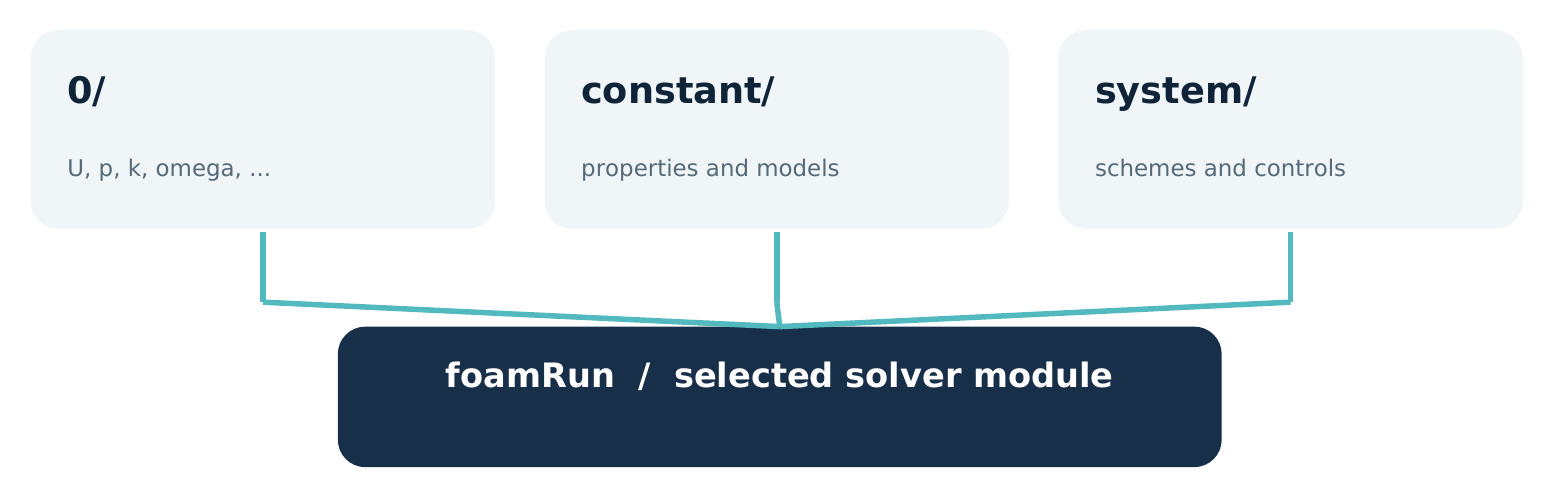
constant/ contains more than a mesh. In Foundation v14 a typical incompressible single-phase case places physical properties in physicalProperties and momentum-transport modelling in momentumTransport.
| Case layer | Question answered | Typical example |
|---|---|---|
0/ | What quantities exist and how are they initialised? | U, p; possibly k, epsilon, omega, nut |
constant/physicalProperties | What material behaviour is provided? | viscosityModel constant; nu ... |
constant/momentumTransport | How is viscous stress / turbulence treated? | simulationType laminar; or RAS model |
system/fvSchemes | How are the equations discretised? | div, grad, laplacian schemes |
system/fvSolution | How are algebraic systems solved? | linear solvers and PIMPLE controls |
Core distinction
A different value of nu is a changed material property. A change from laminar to RAS changes the mathematical closure and usually introduces additional configuration and fields.
Deep dive: who reads constant/ — the solver module, not a generic “OpenFOAM”
In v14 there is a single executable, foamRun, which loads the solver module named by the solver entry in system/controlDict (for this course solver incompressibleFluid;). It is the module that decides which files of constant/ it needs. incompressibleFluid constructs a viscosity model from physicalProperties and a momentum-transport model from momentumTransport; a compressible module such as fluid instead builds a thermophysical package from physicalProperties and reads quite different entries.
You can see this happen at the beginning of the log: after the mesh is read, the module prints lines announcing the selection of the viscosity model and of the momentum-transport model (for a laminar case the selected laminar stress model, by default the Newtonian one). Reading these few lines is the fastest way to confirm that OpenFOAM interpreted your dictionaries as you intended.
foamDictionary system/controlDict -entry solver -value
foamRun 2>&1 | tee log.foamRun
grep -i "select" log.foamRun
The table above is therefore a map of responsibility: if a run fails or gives an unexpected result, the layer that owns the choice is the first place to look. A wrong viscosity is a constant/ problem; a missing initial field is a 0/ problem; a missing div(phi,k) entry is a system/ problem, even if the cause was a decision taken in constant/momentumTransport.
2. Material data: what belongs in physicalProperties?
For the simple isothermal, incompressible channel, the first property of interest is kinematic viscosity, written nu. In the Foundation v14 tutorial case it is provided by a material-property dictionary.
Minimal illustrative constant/physicalProperties
FoamFile
{
    format        ascii;
    class         dictionary;
    object        physicalProperties;
}

viscosityModel    constant;
nu                1e-05;
viscosityModel constant tells OpenFOAM to use a spatially uniform and time-independent kinematic viscosity. nu 1e-05 is 1 × 10⁻⁵ m²/s in the default SI unit system.
The FoamFile header is standard dictionary syntax. The two material entries below the header are the essential content for this example.
Important scope note
Do not infer that every OpenFOAM solver reads only this file or needs these two entries. Compressible, thermal, reacting and multiphase applications use different model packages and may require substantially more configuration.
Worked task / independent check
- In a working case, locate the material property file and identify its
FoamFile/object. - Locate the lines defining the viscosity model and its numerical parameter.
- State which parts of the case would not change if only
nuwere altered.
Deep dive: reading and checking physicalProperties from the command line
Instead of opening the file in an editor, query exactly the entries the solver will read. foamDictionary parses the file with the same reader that OpenFOAM uses, so a syntax error shows up here before a run:
foamDictionary constant/physicalProperties -entry viscosityModel -value
foamDictionary constant/physicalProperties -entry nu -value
foamDictionary constant/momentumTransport -entry simulationType -value
Expected answers for the laminar channel: constant, 1e-05 (or whatever your baseline uses) and laminar. The FoamFile/object entry must be physicalProperties: it is the name under which the file is registered, and it should match the file name.
Answer to task 3. If only nu changes, the mesh (constant/polyMesh), the list of fields in 0/ and their boundary conditions, momentumTransport, fvSchemes, fvSolution and controlDict do not change. What changes is the solution: the viscous term of the momentum equation is multiplied by a different coefficient, so velocity profile development, pressure drop and Reynolds number change. If the case is defined by a fixed velocity at the inlet, the flow rate stays the same and the pressure drop responds; if it were driven by a fixed pressure difference, the flow rate would respond instead.
Typical failure. If nu is misspelt or missing, the run stops while constructing the viscosity model with a fatal IO error stating that keyword nu is undefined in dictionary …/constant/physicalProperties. The message names both the keyword and the file: read it before changing anything else.
Deep dive: v14 units in physicalProperties
The v14 release notes state that physical properties should specify units with the value rather than repeating a dimension set. A plain number is read in the base units of the active unit set (SI by default), so nu 1e-05; means 1 × 10⁻⁵ m²/s. Writing the unit explicitly adds a check and allows conversion on reading:
viscosityModel    constant;
nu                1e-05 [m^2/s];

// equivalent, the value is converted to m^2/s on reading:
// nu             10 [cSt];
Both forms give the same internal value: 10 cSt = 10 × 10−6 m²/s = 1 × 10⁻⁵ m²/s. If you write a unit of the wrong kind (for example [m/s]), the dimension check of the dimensioned property detects the inconsistency. If you write a correct unit with a wrong magnitude, nothing detects it: see section 4.
In older Foundation versions and in many tutorials found online the property was written with an index dimension set, nu [0 2 -1 0 0 0 0] 1e-05;. Read it as “dimensions of m²/s, value 1e-05”; in v14 the preferred style is the bare value or the value followed by a unit.
3. Physics checkpoint: dynamic vs kinematic viscosity
There are two related but different viscosity quantities. They must never be interchanged numerically without accounting for density.
| Quantity | Symbol | SI dimensions | Meaning |
|---|---|---|---|
| Dynamic viscosity | μ | Pa·s = kg/(m·s) | Coefficient between stress and strain rate |
| Kinematic viscosity | ν = μ/ρ | m²/s | Momentum diffusivity per unit density |
| Density | ρ | kg/m³ | Mass per unit volume |
Example. For an illustrative liquid with density 1000 kg/m³ and dynamic viscosity 1.0 × 10⁻³ Pa·s:
Hand calculation (not OpenFOAM syntax)
nu = mu / rho
   = 1.0e-3 / 1000
   = 1.0e-6 m^2/s
Optional refresher / Newtonian fluid
For a Newtonian fluid, the viscous stress depends linearly on the local strain-rate tensor. The molecular viscosity models this material response; the turbulent eddy viscosity introduced by many RAS models is a modelled transport effect, not another tabulated fluid property.
Worked task / independent check
- Convert μ = 1.8 × 10⁻⁵ Pa·s and ρ = 1.2 kg/m³ into ν.
- Identify whether a value stated in centipoise is dynamic viscosity or kinematic viscosity.
- Explain why changing density alone does not imply that the incompressible channel dictionary has a direct density entry.
Deep dive: the Newtonian law and why the incompressible solver needs no density
For a Newtonian fluid the viscous stress is τ = 2μD, where D = ½(∇U + ∇UT) is the strain-rate tensor (for incompressible flow the volumetric part vanishes). With constant density, the momentum equation can be divided by ρ:
dU/dt + div(U U) = -grad(p/rho) + div( 2 (mu/rho) D )
                 = -grad(p_k)    + div( 2 nu D )
Density disappears as an independent parameter: only ν = μ/ρ appears, and the pressure solved for is the kinematic pressure pk = p/ρ, in m²/s². This is why incompressibleFluid reads nu and not rho, and why 0/p in such a case is in m²/s², not Pa. To report a pressure difference in pascal, multiply by the density you assume for the fluid: Δp [Pa] = ρ × Δpk [m²/s²].
Answer to task 3. Changing the density of the real fluid, at the same dynamic viscosity, changes ν. In the incompressible channel that change enters only through nu; there is no separate density entry to edit, and the kinematic pressure field remains independent of ρ until you convert it for reporting.
Useful reference values (approximate, 20 °C, 1 atm): water μ ≈ 1.0 × 10⁻³ Pa·s, ρ ≈ 998 kg/m³, ν ≈ 1.0 × 10⁻⁶ m²/s; air μ ≈ 1.8 × 10⁻⁵ Pa·s, ρ ≈ 1.2 kg/m³, ν ≈ 1.5 × 10⁻⁵ m²/s. Note that air is about 15 times more “viscous” than water in kinematic terms even though its dynamic viscosity is about 55 times lower.
Units of practice. 1 P (poise) = 0.1 Pa·s, so 1 cP = 1 mPa·s = 10−3 Pa·s (dynamic). 1 St (stokes) = 10−4 m²/s, so 1 cSt = 10−6 m²/s (kinematic). Water at about 20 °C is close to 1 cP and 1 cSt, which is the origin of many confusions: the numbers coincide only because ρ ≈ 1000 kg/m³.
4. Units in Foundation v14: use values with dimensional meaning
OpenFOAM checks dimensions to prevent physically invalid combinations. Foundation v14 increasingly uses named dimensions in field files and supports explicit units when reading numerical parameters.
Read the built-in units information
foamUnits
foamUnits pressure
foamUnits kinematicViscosity
A named dimension can appear in a field file as:
Illustrative field metadata
dimensions [kinematicViscosity];A familiar velocity example from the User Guide demonstrates conversion of a value supplied in centimetres per second:
Boundary-condition fragment: 1000 cm/s = 10 m/s
inlet
{
    type    fixedValue;
    value   uniform (1000 0 0) [cm/s];
}
Do not confuse dimension (what physical type of quantity this is) with unit (how its numerical value is expressed). The default numerical units in a simple SI case are usually implicit.
Optional refresher / dimensional consistency
If a field expects viscosity but receives the dimensions of velocity, OpenFOAM can detect the mismatch. If a value has the correct dimensions but the wrong magnitude, the configuration may still run and produce physically incorrect results. Unit checking is necessary, not sufficient.
Deep dive: dimension sets, named dimensions, unit sets and what foamUnits prints
Internally every dimensioned quantity carries a dimension set of seven exponents in the order mass, length, time, temperature, quantity (moles), current, luminous intensity. Kinematic viscosity is [0 2 -1 0 0 0 0]; in v14 the same thing can be written with a name, [kinematicViscosity], or with an expression such as [area/time] or [sqr(length)/time]. The v14 example cases have replaced numerical dimension sets with named ones.
A unit instead says how the number is expressed. Units are written in square brackets after a value ([cm/s], [cm s^-1], [mm], [bar], [cSt], [deg], [%]) and the value is converted to the base units of the active unit set when it is read. The unit sets (SI by default; CGS and USCS are also preconfigured) are defined in the units section of $FOAM_ETC/configDict, and a case can override them in system/configDict.
foamUnits (an application in v14, User Guide §4.7.7) lists dimensions and the units that correspond to them. For pressure the guide shows output of this form:
Dimension [pressure]
+ Dimensions = [mass length^-1 time^-2]
+ Exponents = [1 -1 -2 0 0 0 0]
+ Standard Units = [kg m^-1 s^-2] [Pa]
+ Other Units = [psi] [atm] [kPa] [bar] [MPa]
Running foamUnits kinematicViscosity gives the analogous report: exponents [0 2 -1 0 0 0 0], standard unit m²/s and any other units defined for that dimension in your configuration.
What is checked and what is not. Dimensioned properties and fields compare the supplied unit with the dimensions hard-coded in the solver; plain scalar parameters (a relaxation factor, a tolerance) are not dimension-checked. When two quantities with different dimensions are added or equated, OpenFOAM stops with a fatal error stating that the dimensions differ for the operation (the message shows the two dimension sets). A wrong magnitude — 1e-5 typed as 1e-6, a value in cSt written without the unit — passes every check: compare with an independent hand estimate, as in section 3.
5. Find the source: interrogate an installed v14 tutorial
Use the official Foundation v14 backward-facing-step tutorial as a documentation anchor. The installed path is normally $FOAM_TUTORIALS/incompressibleFluid/pitzDailySteady.
Run from your copied case for the final line
foamVersion
printf "%s\n" "$FOAM_TUTORIALS"
ls "$FOAM_TUTORIALS/incompressibleFluid/pitzDailySteady/constant"

foamDictionary constant/physicalProperties
Compare the actual file against the minimal example. Learn which files are required by the selected solver module, not by all possible OpenFOAM applications.
The case from the official tutorial uses viscosityModel constant and a numerical nu. The same case is turbulent, so its momentum-transport configuration is separate.
Worked task / independent check
- Confirm the environment says OpenFOAM 14.
- Open
constant/physicalPropertiesfrom a working tutorial copy and read its value. - Locate
constant/momentumTransportand record itssimulationType. - Describe in two sentences what would be gained by keeping these choices in separate dictionaries.
Version guard
Avoid copying transportProperties and turbulenceProperties examples from a different OpenFOAM distribution without checking whether their structure applies to Foundation v14.
Deep dive: what you will find in pitzDailySteady
The complete sequence, working on a copy (never inside $FOAM_TUTORIALS):
mkdir -p "$FOAM_RUN"
cp -r "$FOAM_TUTORIALS/incompressibleFluid/pitzDailySteady" "$FOAM_RUN"/
cd "$FOAM_RUN/pitzDailySteady"
ls 0 constant system
foamDictionary system/controlDict -entry solver -value
foamDictionary constant/physicalProperties
foamDictionary constant/momentumTransport
According to the v14 User Guide (§2.1), the tutorial runs the incompressibleFluid module through foamRun; physicalProperties contains viscosityModel constant; and nu 1e-05;; momentumTransport contains simulationType RAS; with model kEpsilon; and turbulence on; (the guide also shows a viscosityModel Newtonian; entry in the RAS settings, the laminar part of the stress, and a comment listing other models tested on this case). 0/ contains U, p, k, epsilon, nut and also omega, so that kOmegaSST can be selected without creating a new file.
The geometry is the Pitz–Daily backward-facing step, with a step height of 25.4 mm and an inlet velocity of 10 m/s. With ν = 1 × 10⁻⁵ m²/s the Reynolds number based on step height is 10 × 0.0254 / 10−5 ≈ 25 400: clearly turbulent, which is why the tutorial uses RAS and not laminar.
Answer to task 4 (one possible formulation). Separating the material from the stress model means a viscosity can be changed without touching the closure, and a closure can be changed without retyping the material data. It also documents the case: anyone can see at once which part is a property of the fluid and which part is a modelling choice.
Deep dive: translating old or ESI-style examples into Foundation v14
Much material online refers to older Foundation releases or to the ESI fork (openfoam.com), whose files have the same purpose but different names and keywords. The mapping below is a guide for reading such examples; always rewrite them in the v14 form and verify with the installed tools.
| Older Foundation / ESI-style | Foundation v14 |
|---|---|
constant/transportProperties | constant/physicalProperties |
transportModel Newtonian; | viscosityModel constant; |
nu [0 2 -1 0 0 0 0] 1e-05; | nu 1e-05; or nu 1e-05 [m^2/s]; |
constant/turbulenceProperties | constant/momentumTransport |
RASModel kEpsilon; / LESModel …; | model kEpsilon; / model …; |
printCoeffs on; | #print |
kEpsilonCoeffs { … } | kEpsilon { … } (or entries directly in RAS) |
simpleFoam, pimpleFoam | foamRun with solver incompressibleFluid; |
The v14 release notes also say that the Coeffs suffix has been removed from the names of model coefficient sub-dictionaries (with backward compatibility). If a copied entry is not recognised, OpenFOAM often does not fail: an unknown keyword in a dictionary is simply ignored, and the model runs with its defaults. That is the most dangerous outcome, because nothing warns you. Use #print (section 14) to see what the model actually read.
6. Momentum transport: the simplest laminar configuration
A Newtonian laminar channel is configured by keeping the baseline viscosity in physicalProperties and selecting no turbulence closure in momentumTransport.
Minimal illustrative constant/momentumTransport
FoamFile
{
    format        ascii;
    class         dictionary;
    object        momentumTransport;
}

simulationType laminar;
For this common case, a laminar sub-dictionary is optional: OpenFOAM defaults to a Newtonian momentum-transport model and obtains nu from the material property file.

This does not mean viscous effects are disabled. Laminar flow still includes viscous stress. It means no turbulence model adds unresolved turbulent transport.
Why it matters
A pressure drop in a laminar channel depends on viscosity and the flow rate, with the expected relation depending on geometry and flow regime. It should not be interpreted as a “turbulence off” pressure loss.
Deep dive: what “laminar” means inside OpenFOAM
simulationType selects one of three branches: laminar, RAS or LES. Within the laminar branch there is again a model selection, made by the optional laminar { model …; } sub-dictionary. When it is absent, the default Newtonian laminar model is used (in the Foundation source code this default class has traditionally been named Stokes, after the linear viscous-stress law; the name printed in the log and by foamToC in your build is authoritative). The other laminar models are the generalised-Newtonian and visco-elastic ones of section 16.
The equations solved by incompressibleFluid in this configuration are continuity and the momentum equation with the stress 2νD and ν taken from physicalProperties. No k, epsilon, omega or nut fields are needed, and if they are present in 0/ they are simply not read.
To list the laminar models available in your build:
foamToC -table laminarincompressibleMomentumTransportModelWorked example for the “why it matters” box. For fully developed flow between parallel plates spaced H, with bulk velocity Ub, the kinematic pressure gradient is −dpk/dx = 12 ν Ub / H². With ν = 1 × 10⁻⁵ m²/s, Ub = 0.1 m/s, H = 0.01 m and a length of 0.1 m: Δpk = 12 × 10−5 × 0.1 / 10−4 × 0.1 = 0.012 m²/s² (12 Pa for a fluid with ρ = 1000 kg/m³). The drop is entirely viscous and proportional to ν — but only in the fully developed part of the channel (see section 20).
7. Optional refresher: what is meant by a closure model?
The Navier–Stokes equations require a representation of stress. For a Newtonian laminar fluid, the molecular viscous stress is linked to resolved velocity gradients through a constitutive relation.
When a RAS model is selected, the equations describe an averaged field and need additional closure for the impact of unresolved velocity fluctuations. A common approach introduces turbulent viscosity and solves auxiliary model equations.
| Model class | Resolved description | Extra modelling |
|---|---|---|
| Laminar Newtonian | Velocity and pressure resolved by the chosen equations | Molecular viscous stress only |
| RAS / RANS | Mean velocity and pressure | Modelled turbulent Reynolds stresses; turbulence fields |
| LES | Large-scale unsteady structures | Subgrid-scale closure plus adequate spatial/time resolution |
Optional refresher / averages
Averaging generates additional terms such as Reynolds stresses. These are not properties of the fluid at rest and therefore do not belong as a tabulated constant in physicalProperties.
Practical consequence
Choosing a model changes which equations and model fields exist. The configuration task extends across the momentumTransport dictionary, field initialisation, boundary conditions, and sometimes numerical settings.
Deep dive: the closure problem in equations
Split the velocity into a mean and a fluctuation and average the momentum equation. The non-linear convective term produces a new unknown, the Reynolds stress tensor ⟨u′u′⟩: six additional unknown components with no additional equation. This is the closure problem.
U = <U> + u'                         (Reynolds decomposition)

d<U>/dt + div(<U><U>) = -grad(<p>) + div[ 2 nu D(<U>) ] - div( <u'u'> )

-<u'u'> = 2 nut D(<U>) - (2/3) k I   (Boussinesq hypothesis)

nuEff = nu + nut
The Boussinesq hypothesis models the Reynolds stresses as an extra viscous stress with a turbulent (eddy) viscosity νt, which is a property of the flow, not of the fluid: it varies in space and time, can be hundreds of times larger than ν in a turbulent core and goes to zero at a wall. The momentum equation then has the same form as the laminar one with ν replaced by νeff = ν + νt. The RAS model’s job is to compute νt, usually from one or two additional transported scalars (k and ε, k and ω, or ν̃).
In OpenFOAM this is visible in the field names: nut is νt, stored as a field with its own boundary conditions; the effective viscosity nuEff appears in the names of some terms of fvSchemes. LES uses the same idea at a different scale: the filtered equations contain a subgrid stress modelled with a subgrid viscosity, and the large eddies are resolved in time rather than averaged away.
8. Flow regime: use the Reynolds number as a guide
A model should be selected because the physical problem demands it, not because it is available in a drop-down list or another case uses it.
Dimensionless flow scale: definition
Re = U_ref * L_ref / nuWorked illustration: U = 0.20 m/s, characteristic channel height L = 0.010 m and ν = 1.0 × 10⁻⁶ m²/s give Re = 2000. The threshold for transition depends on geometry, disturbances and how the characteristic scales are defined.
This number is not an automatic switch between laminar and turbulent settings for all flows. For the channel case, record the chosen characteristic length and compare with an appropriate reference for that geometry.
| Change | Effect if other quantities fixed |
|---|---|
| Double the characteristic velocity | Re doubles |
| Double the length scale | Re doubles |
| Double kinematic viscosity | Re halves |
| Change geometry / inlet disturbances | May change transition mechanisms and appropriate model |
Worked task / independent check
- Compute Re for U = 0.05 m/s, L = 0.008 m, ν = 1.0 × 10⁻⁶ m²/s.
- Explain whether the result alone proves the flow is fully developed.
- Document why you would retain a laminar model for a low-Re teaching case.
Deep dive: which length, which velocity, which threshold
A Reynolds number is meaningful only together with its definition. For internal flows the usual choice is the bulk (mean) velocity and the hydraulic diameter Dh = 4A/P (A cross-section area, P wetted perimeter). For a circular pipe Dh = D; for two infinite parallel plates spaced H, Dh = 2H; for the 10 mm × 5 mm duct of Part 2, Dh = 4 × 50 / 30 ≈ 6.67 mm. Using the channel height instead of Dh changes Re by a factor of two for plates: the Re = 2000 based on H used here would be Re = 4000 based on Dh.
The classical reference values are therefore not interchangeable: about 2300 for a pipe (bulk velocity, diameter) as the usual lower bound of transition; for plane channel flow, linear stability theory gives about 5772 based on centreline velocity and half-height, while in experiments transition can occur at considerably lower values when disturbances are present. Inlet disturbances, roughness and the shape of the inlet profile all move the actual threshold.
Fully developed is a different question. Re says nothing about the distance needed for the profile to stop changing. For laminar internal flow the entrance length grows with Re; a common estimate for pipes is Le ≈ 0.05 Re Dh. At Re = 400 and Dh = 8 mm this already gives about 0.16 m: a short channel may never be fully developed. Check it in the solution by comparing velocity profiles at two stations, not by Re.
Answer to task 3. At low Re, with a physically laminar flow, a laminar model is not a simplification but the correct physics: there are no turbulent fluctuations to model, the solution can be compared with an analytical one (Poiseuille), and adding a RAS model would introduce a turbulent viscosity that does not exist, extra fields and extra uncertainty.
9. RAS model selection: the momentumTransport RAS branch
In a Reynolds-averaged simulation, simulationType RAS activates a sub-dictionary named RAS. In Foundation v14, the model name is specified by model.
Configuration fragment (not a standalone runnable case)
simulationType RAS;

RAS
{
      model            kEpsilon;
      turbulence       on;
}
The turbulence switch controls solving the turbulence model. The model choice and its coefficients can be configured in this dictionary.
Verify available models and example usage in v14
foamToC -table RASincompressibleMomentumTransportModel
foamSearch "$FOAM_TUTORIALS" momentumTransport RAS/model
Model change is not one line
The fragment above does not provide 0/k, 0/epsilon, or 0/nut; it is a map of the model branch. Do not insert it into a laminar case and assume the case is complete.
Deep dive: the standard k–ε model and what the two commands print
The standard k–ε model transports the turbulent kinetic energy k (m²/s²) and its dissipation rate ε (m²/s³) and builds the eddy viscosity from them:
nut = Cmu * k^2 / epsilon

Dk/Dt       = div[ (nu + nut/sigmak)   grad(k) ]       + G - epsilon
Depsilon/Dt = div[ (nu + nut/sigmaEps) grad(epsilon) ] + C1*G*epsilon/k - C2*epsilon^2/k

G = nut * 2 |symm(grad(U))|^2

standard constants: Cmu = 0.09, C1 = 1.44, C2 = 1.92, sigmak = 1.0, sigmaEps = 1.3
G is the production of k by the mean shear. The constants are those of the standard model; in OpenFOAM they are defaults in the implementation and are printed with #print (section 14).
foamToC -table RASincompressibleMomentumTransportModel prints the names registered in that run-time selection table. According to the v14 User Guide the incompressible RAS list includes LRR, LamBremhorstKE, LaunderSharmaKE, LienCubicKE, LienLeschziner, RNGkEpsilon, SSG, ShihQuadraticKE, SpalartAllmaras, kEpsilon, kEpsilonLopesdaCosta, kOmega, kOmega2006, kOmegaSST, kOmegaSSTLM, kOmegaSSTSAS, kkLOmega, qZeta, realizableKE and v2f. Your installation is the final authority. foamSearch "$FOAM_TUTORIALS" momentumTransport RAS/model instead scans all momentumTransport files of the tutorials and prints the distinct values of the RAS/model entry: it tells you which models are actually used in official examples.
turbulence off. With turbulence off; the model equations are not solved, so k, ε and νt keep the values they have. It is a tool for special procedures (for example initialising a flow field), not a way to obtain a laminar simulation: for that, use simulationType laminar.
10. Model-to-field dependency: what a k–epsilon case must initialise
The standard kEpsilon RAS model introduces transport equations for turbulent kinetic energy k and its dissipation rate epsilon. A typical Foundation v14 tutorial case also configures a turbulent-viscosity field nut for appropriate boundaries.
| File | Typical meaning | What to inspect |
|---|---|---|
0/U | Mean velocity | inlet, outlet, walls |
0/p | Mean kinematic pressure for this incompressible formulation | outlet/reference and gradients |
0/k | Turbulent kinetic energy | internal value, inlet and wall treatment |
0/epsilon | Turbulent kinetic-energy dissipation | initial/inlet and wall functions |
0/nut | Turbulent kinematic viscosity | calculated values and wall functions |
In addition, the field entries must be supported by the numerical terms in fvSchemes and the linear-solvers / algorithm controls in fvSolution. Model fields are not merely visualisation outputs.
Do not invent a generic BC recipe
The precise inlet and wall conditions depend on the chosen RAS model, turbulence intensity, wall treatment and resolved near-wall mesh. Consult a relevant official v14 tutorial before copying an entry.
Deep dive: dimensions and boundary conditions of the turbulence fields
Each new file must have the right dimensions and a boundary condition for every patch of the mesh:
| Field | Dimensions (exponents) | SI unit |
|---|---|---|
k | [0 2 -2 0 0 0 0] | m²/s² |
epsilon | [0 2 -3 0 0 0 0] | m²/s³ |
omega | [0 0 -1 0 0 0 0] | 1/s |
nut | [0 2 -1 0 0 0 0] (named [turbulentViscosity]) | m²/s |
nuTilda | [0 2 -1 0 0 0 0] | m²/s |
In pitzDailySteady, as described by the v14 guide: k and epsilon have internal and inlet values 0.375 and 14.855; on the walls k uses kqRWallFunction, epsilon uses epsilonWallFunction and nut uses nutkWallFunction; nut is calculated on inlet and outlet; frontAndBack is empty for all fields because the case is two-dimensional. Read the outlet conditions of k and epsilon in your copy (an outflow condition that switches to a fixed value if backflow occurs is the usual pattern).
The v14 release notes also report that the inlet turbulence boundary conditions have been simplified into turbulentKineticEnergy, turbulentEpsilon and turbulentOmega, which, as their names and the conditions they replace suggest, derive inlet values from turbulence-intensity and length-scale (or mixing-length) assumptions. Check their actual parameters with foamInfo turbulentKineticEnergy before using them.
A k–ε run additionally needs entries such as these (illustrative pattern; compare with your copy of pitzDailySteady):
// system/fvSchemes - entries a k-epsilon run additionally needs (illustrative)
divSchemes
{
    // ... existing entries of the case ...
    div(phi,k)          bounded Gauss limitedLinear 1;
    div(phi,epsilon)    bounded Gauss limitedLinear 1;
}

// system/fvSolution - the turbulence fields need a linear solver
solvers
{
    // ... existing p and U entries ...
    "(k|epsilon)"
    {
        solver          smoothSolver;
        smoother        symGaussSeidel;
        tolerance       1e-05;
        relTol          0.1;
    }
}
In a steady SIMPLE case the turbulence fields also usually have relaxation factors and residual controls in fvSolution: see Part 6.
11. An alternative RAS closure: k–omega SST and other choices
The RAS catalogue includes numerous closures. As a second example, kOmegaSST uses different auxiliary fields from kEpsilon.
Model selection only
simulationType RAS;
RAS
{
    model           kOmegaSST;
    turbulence      on;
}| Example RAS family | Common transported fields | Implication |
|---|---|---|
kEpsilon | k and epsilon | Configure k, epsilon and appropriate wall functions |
kOmegaSST | k and omega | Configure k, omega and appropriate wall functions |
SpalartAllmaras | nuTilda | Different model field and boundary requirements |
Even when two models can run on the same mesh, equal values of their parameters do not mean equivalent physics. A meaningful comparison requires physical rationale, adequate near-wall mesh, and appropriate observables.
Worked task / independent check
- Find official v14 examples using
kOmegaSSTwithfoamSearch. - Identify a field which appears in a
kEpsiloncase but is replaced in akOmegaSSTcase. - List what besides
momentumTransportyou would inspect before changing models.
Deep dive: k–ω SST, Spalart–Allmaras and how to find the examples
k–ω SST transports k and the specific dissipation rate ω (1/s), related to ε by ω = ε/(Cμ k). It blends a k–ω formulation near walls with a k–ε-like behaviour away from them and limits the eddy viscosity in strong adverse pressure gradients (the “shear-stress transport” limiter). Its wall treatment uses omegaWallFunction on omega. Spalart–Allmaras is a one-equation model for a modified viscosity ν̃ (nuTilda), from which νt is computed; its boundary conditions are of a different kind (no k, no ε/ω).
Finding the examples. foamSearch lists the distinct values of an entry and how often they occur, which confirms that kOmegaSST is used; to get the actual tutorial paths, search the files, or ask foamInfo, which also lists example cases:
foamToC -help
foamToC -table RAS
foamToC -scalarBCs | grep -i wallfunction
grep -rl --include=momentumTransport kOmegaSST "$FOAM_TUTORIALS"
Answer to task 2. epsilon is replaced by omega; k and nut remain but their boundary conditions must be checked again. Answer to task 3: the fields in 0/ and their boundary conditions (especially walls and inlet), fvSchemes (new div(phi,omega)), fvSolution (solver, relaxation, residual control for omega), the near-wall mesh (y+) and the observables you will compare.
A concrete warning from the official tutorial. The v14 guide reports that on pitzDailySteady the kEpsilon run converges in 285 iterations and realizableKE in 255, while kOmegaSST with the same numerics does not converge and runs to the end time (2000); it converges in 285 iterations only after changing the gradient scheme of U to cellLimited. Same mesh, same case, different model: the numerical settings had to change too.
12. Turbulence initial values: how are k and epsilon estimated?
The model fields need dimensionally and physically meaningful initial and boundary conditions. A common entry point is a specified mean inlet speed and an estimate of turbulence intensity.
Common kinetic-energy estimate
k = 1.5 * (U * I)^2Here U is a characteristic mean speed and I is turbulence intensity as a fraction (5% = 0.05). The estimate is a modelling assumption, not a universal boundary law.
For U = 2.0 m/s and I = 0.05, we obtain k = 0.015 m²/s².
A frequently used dissipation estimate is based on a turbulence length scale l and the coefficient Cμ; its precise suitability depends on the model and flow.
Conceptual model estimate, not dictionary syntax
epsilon = (Cmu^0.75) * (k^1.5) / lOptional refresher / boundary uncertainty
Unlike the molecular viscosity, turbulence intensity and turbulent length scale describe the flow entering the domain. They should be justified by measurements, upstream geometry, empirical estimates or a documented sensitivity analysis.
Worked task / independent check
- Recompute k for U = 1.5 m/s and I = 0.03.
- Describe what is physically uncertain when I is guessed.
- Explain why k cannot simply be copied from the fluid viscosity parameter.
Deep dive: the complete set of estimates and the pitzDailySteady numbers
Where the k = 3/2 (U I)² formula comes from: with isotropic fluctuations u′ = v′ = w′ = U I, k = ½(u′² + v′² + w′²) = 3/2 (U I)². The other quantities follow from k and a length scale l:
epsilon = Cmu^0.75 * k^1.5 / l
omega   = k^0.5 / (Cmu^0.25 * l)  =  epsilon / (Cmu * k)
nut     = Cmu * k^2 / epsilon
(Cmu = 0.09)
Continuing the example above (U = 2.0 m/s, I = 0.05, k = 0.015 m²/s²) with an assumed l = 1 mm: ε ≈ 0.302 m²/s³, ω ≈ 224 1/s, νt ≈ 6.7 × 10⁻⁵ m²/s, that is about 67 times the viscosity of water. A frequently quoted rule for fully developed internal flow takes l ≈ 0.07 Dh; it is an empirical rule of thumb, to be justified like I.
Reverse-engineering the official tutorial. pitzDailySteady has U = 10 m/s and k = 0.375 m²/s²: 1.5 (10 I)² = 0.375 gives I = 0.05 (5%). Its ε = 14.855 m²/s³ gives l = 0.090.75 × 0.3751.5 / 14.855 ≈ 0.00254 m, i.e. one tenth of the 25.4 mm step height; and ω = 14.855/(0.09 × 0.375) ≈ 440.2 1/s, exactly the value the guide reports for 0/omega. The tutorial values are therefore consistent with I = 5% and l = 2.54 mm.
Answer to task 2. I describes the fluctuations of the incoming flow: it depends on what is upstream (a long pipe, a fan, a honeycomb, a contraction) and is rarely measured. Guessing it fixes k at the inlet, and through l also ε or ω and so νt; the downstream development, transition and separation can depend on it. Answer to task 3: k is a property of the flow (energy of velocity fluctuations, m²/s²), ν is a property of the fluid (m²/s): different dimensions and different physical meaning, so neither can be derived from the other.
13. Near-wall modelling: wall functions belong to field BCs
Wall functions are applied on wall patches through turbulence fields, not by changing the mesh patch to a new physical material.
Example fragment inside 0/nut boundaryField
walls
{
    type     nutkWallFunction;
    value    uniform 0;
}
For a kEpsilon-type RAS configuration, related wall conditions are often specified on epsilon and k. The Foundation v14 guide identifies epsilonWallFunction and kqRWallFunction as important available classes.
Wall-function suitability depends on wall-normal resolution. Do not assume wall functions excuse an unvalidated near-wall mesh. The dimensionless distance y+ helps assess wall resolution and compatibility with the selected wall treatment.
Optional refresher / y+
y+ = uτ y / ν, where uτ is friction velocity and y the wall-normal distance of the first cell centre. Values must be interpreted for the actual wall treatment, flow and model; a universal target is not appropriate.
Worked task / independent check
- Identify the wall patch name in
0/nutand compare it toconstant/polyMesh/boundary. - Check which files hold wall functions for your chosen RAS model.
- Explain why the same
0/nutentry should not be reused blindly after switching turbulence model.
Deep dive: the law of the wall, y+ and how to compute it in v14
Near a smooth wall the mean velocity, scaled by the friction velocity uτ = √(τw/ρ), follows a universal profile in the variable y+: a viscous sublayer (u+ ≈ y+, roughly y+ < 5), a buffer layer, and a logarithmic layer (u+ = (1/κ) ln(E y+), with κ ≈ 0.41 and E ≈ 9.8, roughly from y+ ≈ 30 upwards). A wall function uses this law to supply the wall shear stress and the near-wall values of the turbulence quantities when the first cell is too coarse to resolve the gradient.
In OpenFOAM the wall function is a boundary condition: nutkWallFunction computes νt at the wall from k; epsilonWallFunction (or omegaWallFunction) sets the near-wall dissipation; kqRWallFunction is essentially a zero-gradient condition for k. The v14 guide lists the νt wall functions nutWallFunction, nutRoughWallFunction, nutUSpaldingWallFunction, nutkWallFunction and nutkAtmWallFunction; the constants E, κ and Cμ can be overridden per boundary condition. Check the exact names in your build with foamToC -scalarBCs | grep -i wallfunction.
Worked example. If τw/ρ = 0.25 m²/s², then uτ = 0.5 m/s; with ν = 1 × 10⁻⁵ m²/s and the first cell centre at y = 0.5 mm, y+ = 0.5 × 5 × 10−4 / 10−5 = 25. To compute y+ on a result, the post-processing function must be able to construct the momentum-transport model, so run it through the solver module:
foamPostProcess -solver incompressibleFluid -func yPlus -latestTime
foamPostProcess -solver incompressibleFluid -func wallShearStress -latestTime
Answer to task 3. A 0/nut written for kEpsilon assumes that k exists and that the wall treatment is consistent with the first-cell y+ of that mesh; after switching to SpalartAllmaras (no k) or to a low-Re treatment requiring y+ ≈ 1, the same entries are wrong or inconsistent even if the case starts. The patch names in 0/nut must also match constant/polyMesh/boundary exactly (task 1), otherwise the run stops reporting that no patchField entry exists for that patch.
14. RAS coefficients: defaults, overrides and traceability
Turbulence models contain empirical coefficients. Foundation v14 supplies defaults in the implementation. An optional override should have a documented reason and should not be mistaken for a material property.
v14 introspection: print model dictionary and defaults
simulationType RAS;
RAS
{
    model          kEpsilon;
    turbulence     on;
    #print
}
The new and updated v14 dictionary introspection mechanisms make it possible to expose effective defaults for certain model dictionaries. Use #print in a copy of a compatible case and inspect output or expansion; do not add overrides merely because a value exists.
Model coefficients can be supplied directly in the relevant sub-dictionary or, when appropriate, within a further model-named sub-dictionary. The v14 syntax should be verified against the exact model.
Practical standard
For a research case, log: model name, model family, OpenFOAM version, coefficient overrides (if any), wall treatment, turbulence inlet assumptions and the reference used. An undocumented model choice makes later comparisons difficult.
Deep dive: what #print shows and how an override is written
#print is a v14 dictionary directive: placed at the end of a dictionary, it makes OpenFOAM print the dictionary as it is used, including the default entries you did not write. According to the v14 release notes it replaces the writeOptionalEntries function object; in older releases the per-model printCoeffs switch served a similar purpose for model coefficients. In the RAS dictionary of a kEpsilon case it reveals the default coefficients (for example Cmu 0.09;); the same directive inside a PIMPLE dictionary reveals defaults such as nCorrectors 1;. Run the case (a single iteration is enough) and read the printed dictionary at the start of the log. The guide also mentions expanding the file with foamDictionary as an alternative.
If an override is justified, write it in the RAS dictionary or in a sub-dictionary named after the model (in v14 without the old Coeffs suffix):
RAS
{
    model           kEpsilon;
    turbulence      on;

    kEpsilon                // optional, only for a documented override
    {
        Cmu         0.09;
    }
}
Then run again with #print and verify that the printed value is yours: an override with a misspelt keyword is silently ignored. Coefficients are not properties of the fluid: changing Cμ recalibrates the model, and every result obtained with it must say so.
15. LES overview: a different modelling assumption
Foundation v14 also provides LES (large-eddy simulation). Its purpose differs from RAS: larger turbulent structures are resolved as time-dependent motions, while smaller motions receive a subgrid-scale closure.
Schematic only: replace … with a compatible model and delta
simulationType LES;

LES
{
      model        ...;
      turbulence   on;
      delta        ...;
}
An LES dictionary requires compatible model and filter-width/delta settings, plus suitable boundary conditions, time resolution and mesh design. A RAS mesh that converges acceptably is not automatically an LES-quality mesh.
For the reference channel in this course, the laminar baseline remains the recommended learning object. LES is presented to teach how to recognise the configuration architecture, not to require a validated LES simulation.
| Laminar | RAS | LES |
|---|---|---|
| Molecular stress closure | Modelled mean turbulent transport | Time-resolved large structures + subgrid model |
| Relatively small config | Extra turbulence fields | Different fields and delta settings |
| Appropriate for laminar physics | Appropriate with a validated closure | Computationally demanding, especially near walls |
Deep dive: filter width, subgrid models and why LES is expensive
LES applies a spatial filter of width Δ to the equations. Motions larger than Δ are computed; the effect of the smaller ones appears as a subgrid stress, modelled for example with a subgrid viscosity. In the Smagorinsky model νsgs = (Cs Δ)² |S|, with |S| the magnitude of the resolved strain rate; WALE, kEqn, dynamicKEqn and dynamicLagrangian are other choices listed by the v14 guide, together with the hybrid RAS/LES models SpalartAllmarasDES, SpalartAllmarasDDES, SpalartAllmarasIDDES and kOmegaSSTDES, and DeardorffDiffStress.
In OpenFOAM the filter width is itself a run-time-selected delta model, named by the delta entry; the guide gives cubeRootVol (Δ from the cube root of the cell volume) as an example, with its coefficients in a sub-dictionary named after it. The LES dictionary therefore needs model, turbulence, delta and, as needed, model- and delta-named sub-dictionaries. Find working combinations with foamSearch "$FOAM_TUTORIALS" momentumTransport LES/model and foamSearch "$FOAM_TUTORIALS" momentumTransport LES/delta, and list the models with foamToC -table LESincompressibleMomentumTransportModel.
Why it is demanding: LES is always three-dimensional and unsteady; the time step must keep the Courant number low enough to follow the eddies; inflow boundaries must supply realistic fluctuations; results are statistics, accumulated over many flow-through times (for example with a field-averaging function); near walls the energy-carrying eddies become very small, so a wall-resolved LES needs a mesh far finer than a RAS mesh. That is why the course keeps the laminar channel as its learning object.
16. Non-Newtonian behaviour: viscosity can depend on shear rate
Not every fluid behaves as a Newtonian liquid. For some materials, apparent viscosity changes with strain rate. Foundation v14 places such effects in the momentumTransport modelling hierarchy, rather than treating them as an ordinary tabulated fluid-at-rest property.
Model branch only: intentionally incomplete
simulationType laminar;

laminar
{
    model           generalisedNewtonian;
    viscosityModel BirdCarreau;
    // model parameters are required here
}
The physicalProperties dictionary still provides a reference viscosity. For several non-Newtonian models this serves as the zero-shear viscosity, while model-specific coefficients determine the rate-dependent response.
The source documentation lists common examples including BirdCarreau, CrossPowerLaw, powerLaw and HerschelBulkley. Each has different parameters; do not substitute parameters between models merely because a keyword is similar.
Optional refresher / rheology
Shear thinning means apparent viscosity decreases as the characteristic shear rate rises. Yield-stress models add a different constitutive assumption. These are material-behaviour models, not turbulence models.
Deep dive: the generalised-Newtonian laws and their parameters in v14
A generalised-Newtonian model keeps the form τ = 2ν(γ̇)D but lets the viscosity depend on the local strain rate γ̇. The v14 guide (§8.3) describes these laws; the zero-strain-rate viscosity ν0 is the nu of physicalProperties:
strain rate:     gammaDot = sqrt(2) * |symm(grad(U))|

BirdCarreau:     nu = nuInf + (nu0 - nuInf) * [1 + (k*gammaDot)^a]^((n - 1)/a)     (a = 2 by default)
CrossPowerLaw:   nu = nuInf + (nu0 - nuInf) / [1 + (m*gammaDot)^n]
powerLaw:        nu = k * gammaDot^(n - 1),          limited to nuMin <= nu <= nuMax
HerschelBulkley: nu = min( nu0, (tau0 + k*gammaDot^n) / gammaDot )| viscosityModel | Parameters in the laminar dictionary |
|---|---|
BirdCarreau | nuInf, k, n (plus the exponent a) |
CrossPowerLaw | nuInf, m, n |
powerLaw | nuMax, nuMin, k, n |
HerschelBulkley | tau0, k, n |
Casson | m, tau0, nuMax, nuMin |
strainRateFunction | function: ν(γ̇) given with Function1 syntax (e.g. polynomial) |
Notice that k and n appear in several models with different meanings and dimensions (a time constant in BirdCarreau, a consistency index in powerLaw and HerschelBulkley): this is exactly the trap warned about above. A complete illustrative branch, with arbitrary numbers that do not describe a real material:
// constant/physicalProperties: nu is the zero-strain-rate viscosity nu0
viscosityModel  constant;
nu              1e-03;

// constant/momentumTransport (illustrative values, not a material)
simulationType  laminar;

laminar
{
    model           generalisedNewtonian;
    viscosityModel  BirdCarreau;

    nuInf           1e-05;
    k               1;
    n               0.5;
}
Beyond generalised-Newtonian fluids, the laminar branch also contains visco-elastic models (Maxwell, Giesekus, PTT, with parameters such as nuM and lambda) and the lambdaThixotropic model; the v14 release notes add multi-mode visco-elastic models with several relaxation times. The available viscosity laws are listed by foamToC -table generalisedNewtonianViscosityModel.
The same viscosityModel entry also exists in the RAS and LES dictionaries, where it describes the laminar (molecular) part of the stress: it is Newtonian by default, which is why the v14 guide shows viscosityModel Newtonian; in the pitzDailySteady RAS settings and notes that it could be omitted. Rheology and turbulence closure are therefore two independent choices that can be combined.
17. Model availability: ask the installation, not your memory
The official guide shows how to query the v14 runtime-selection tables. This is safer than relying on old internet examples.
Run under a correctly sourced OpenFOAM 14 shell
foamToC -table laminarincompressibleMomentumTransportModel
foamToC -table generalisedNewtonianViscosityModel
foamToC -table RASincompressibleMomentumTransportModel
foamToC -table LESincompressibleMomentumTransportModel
These tables allow you to learn which classes are available in the installed build. The table names reflect the physical and numerical family. A model in a compressible runtime table should not automatically be assumed available in the incompressible case.
Find tutorial usages and documentation
foamSearch "$FOAM_TUTORIALS" momentumTransport RAS/model
foamInfo kEpsilon
Compatibility boundary
Before using a non-Newtonian, viscoelastic, RAS or LES model, verify the selected solver module supports that specific class. Availability of a model somewhere in the installation does not guarantee compatibility with every module.
Worked task / independent check
- List available incompressible laminar transport models.
- Find two different RAS models in the table.
- Locate one official tutorial demonstrating the chosen model.
Deep dive: run-time selection tables and the error you get from a wrong name
OpenFOAM builds models by name at run time: each family has a run-time selection table that maps a word (kEpsilon) to a class. The table name encodes the family — RAS + incompressible + MomentumTransportModel — which is why a compressible model is in a different table (the guide shows, for example, buoyantKEpsilon only among the compressible RAS models). foamToC -help lists the other options of the tool; foamToC -table RAS is the form the guide uses to search for tables whose name contains RAS.
If you write a name that is not in the table, the run stops with a fatal error stating that the type is unknown, followed by the list of valid types (the exact wording depends on the build): the error message is itself a foamToC listing, filtered by the module actually running. It is the definitive answer to “does this module support this model?”.
foamInfo kEpsilon prints the description from the source header, the location of the source files and a list of tutorials that use the model: the quickest answer to task 3. foamSearch works on the files of a directory tree and is the right tool to see which values are used in practice.
18. Beyond isothermal incompressible: thermophysical configuration is another layer
Thermal, compressible, multicomponent and reacting simulations need additional physical data and often an expanded physicalProperties dictionary. This is intentionally outside the hands-on channel exercise.
v14 guide example: structural illustration only
thermoType
{
    type            hePsiThermo;
    mixture         pureMixture;
    transport       const;
    thermo          hConst;
    equationOfState perfectGas;
    specie          specie;
    energy          sensibleEnthalpy;
}
These entries select a thermophysical package: equation of state, mixture, transport correlations, thermodynamic model and energy variable. The requirements are tied to the actual solver module.
Do not paste this example into the laminar incompressible channel: it represents a different physical system and application family.
Optional refresher / thermophysical models
In a compressible fluid, density and other properties may depend on pressure, temperature and composition. A constant kinematic viscosity model alone cannot represent that entire behaviour.
Deep dive: reading a thermoType entry by entry
In a compressible or thermal module (for example fluid), physicalProperties describes a whole thermophysical package. Each entry of thermoType selects one ingredient; the options below are those listed by the v14 guide (§8.1):
| Entry | Meaning | Options in the v14 guide |
|---|---|---|
type | Overall thermo class: how density is obtained | hePsiThermo (compressibility ψ, ρ = ψp), heRhoThermo, heheuPsiThermo, heSolidThermo |
mixture | Single species or mixture | pureMixture, multicomponentMixture, coefficientWilkeMulticomponentMixture, valueMulticomponentMixture, homogeneousMixture, inhomogeneousMixture, veryInhomogeneousMixture |
transport | Viscosity and conductivity law | const, sutherland, polynomial, logPolynomial, Andrade, tabulated, icoTabulated, WLF |
thermo | Heat capacity / enthalpy model | hConst, eConst, janaf, hPolynomial, ePolynomial, hPower, ePower, hTabulated, eTabulated, hIcoTabulated, eIcoTabulated |
equationOfState | ρ(p, T) | perfectGas, rhoConst, incompressiblePerfectGas, Boussinesq, perfectFluid, PengRobinsonGas, linear, adiabaticPerfectFluid, icoPolynomial, icoTabulated, rhoTabulated, rPolynomial |
specie | Molecular data | specie |
energy | Energy variable solved | sensibleEnthalpy, sensibleInternalEnergy, absoluteEnthalpy (examples given by the guide) |
The package then needs the data for the chosen ingredients, grouped in a sub-dictionary: molecular weight, heat capacity and heat of formation, dynamic viscosity and Prandtl number for const transport. An illustrative structure for air:
mixture
{
    specie
    {
        molWeight       28.96;
    }
    thermodynamics
    {
        Cp              1004.5;
        Hf              0;
    }
    transport
    {
        mu              1.8e-05;
        Pr              0.7;
    }
}
Note that here the transport property is the dynamic viscosity mu (Pa·s), not nu: in a compressible module density is a field, so the kinematic shortcut of section 3 is no longer available. With transport sutherland, μ also becomes a function of temperature. A fresh compressible case also needs a temperature field 0/T, a pressure in pascal and thermal boundary conditions.
19. Case dependency audit: what changes when physics changes?
| Proposed change | Files to review | Reason |
|---|---|---|
| Change ν only | constant/physicalProperties | Material momentum diffusivity changes |
| Laminar → kEpsilon RAS | momentumTransport; 0/k, 0/epsilon, 0/nut; 0/U, 0/p; fvSchemes; fvSolution | Closure and additional equations/BCs |
| kEpsilon → kOmegaSST | momentumTransport; 0/k, 0/omega, 0/nut; numerical controls and wall BCs | Different auxiliary field/BC requirements |
| Newtonian → BirdCarreau | physicalProperties and momentumTransport; output/validation | Reference viscosity and rheological law change |
| Isothermal → thermal/compressible | Selected solver; physicalProperties thermoType; new fields; BCs; numerics | Different governing equations and properties |
The exact list of files depends on the chosen module and version. The table is a review checklist, not an auto-generated case template.
Golden rule
Whenever you change the physical model, ask: What equations changed? What unknowns were added? Which initial and boundary data are now required? Which numerical settings must be extended?
Deep dive: doing the audit with tools instead of memory
The fastest way to see what a physics change touches is to compare a case that already has it. Copy a laminar case and a RAS tutorial and diff their structures:
ls 0 constant system
diff <(ls ../laminarCase/0) <(ls 0)
foamDictionary system/fvSchemes -entry divSchemes
foamDictionary system/fvSolution -entry solvers -keywords
-keywords prints only the keywords of a dictionary, which shows at a glance which fields have a linear solver. Answer the four questions of the golden rule in writing for each row of the table. For laminar → kEpsilon, for example: (1) two transport equations for k and ε are added and the momentum equation uses ν + νt; (2) the unknowns k, ε and the derived field νt are added; (3) initial and inlet values of k and ε, wall functions on every wall, outlet conditions; (4) div(phi,k), div(phi,epsilon), solvers and, for SIMPLE, relaxation and residual controls for the new fields.
For “Newtonian → BirdCarreau”, the extra word “output/validation” in the table is important: with a shear-thinning fluid the analytical Poiseuille solution no longer applies, so the comparison you used to validate the laminar channel must be replaced by an appropriate reference.
20. Experiment A: controlled viscosity experiment
This experiment is intended to be executable with the already working laminar reference channel from the previous parts (the laminar channel case). Do not change the mesh, inlet BC, time settings, numerical schemes or solver controls during the comparison.
Prepare three copies
Replace channelBaseline with your own working case directory
cp -a channelBaseline channel_nu_base
cp -a channelBaseline channel_nu_half
cp -a channelBaseline channel_nu_double
Set the material viscosity in the copies as follows:
| Run | nu (m²/s) | Hypothesis |
|---|---|---|
| BASE | 1.0 × 10⁻⁵ | Reference viscous response |
| HALF | 5.0 × 10⁻⁶ | Lower molecular viscous diffusion |
| DOUBLE | 2.0 × 10⁻⁵ | Higher molecular viscous diffusion |
If the original case has a different reference viscosity, preserve its original value for BASE and use exactly half/twice that actual value in the two variants.
Interpretation warning
Do not assert that pressure loss must change by exactly a factor of two unless the assumptions of that scaling are verified (e.g. fully developed laminar conditions, fixed flow rate and suitable geometry). The purpose is to compare measured outputs and explain the regime.
Deep dive: setting the values without an editor and checking that nothing else changed
cp -a copies the whole directory preserving timestamps and permissions. If channelBaseline already contains result time directories, remove them in each copy (foamListTimes -rm, run inside the copy) so that all three runs start from the same 0/. Then set the values with foamDictionary and verify:
foamDictionary channel_nu_half/constant/physicalProperties   -entry nu -set 5e-06
foamDictionary channel_nu_double/constant/physicalProperties -entry nu -set 2e-05

for c in channel_nu_base channel_nu_half channel_nu_double
do
    printf "%-20s nu = %s\n" "$c" "$(foamDictionary $c/constant/physicalProperties -entry nu -value)"
done

diff -r channel_nu_base/constant channel_nu_half/constant
The diff -r output must show only the nu line. Anything else is an uncontrolled change and invalidates the comparison.
What theory predicts, and when. In the fully developed region of a laminar channel at fixed flow rate, the kinematic pressure gradient is proportional to ν (12 ν Ub/H² for plates, the analogous Hagen–Poiseuille law for a pipe), so HALF and DOUBLE should give about half and twice the BASE gradient there. The total inlet-to-outlet difference also contains the developing region, where the excess pressure loss depends on Re: with ν halved, Re doubles and the entrance length grows, so the total ratio can deviate from 2. If the inlet were a fixed pressure difference instead of a fixed velocity, the flow rate would change instead. These are the reasons for the interpretation warning.
21. Experiment A continued: run, measure and report
Example workflow; repeat for each copied case
cd channel_nu_base
blockMesh             # only if mesh not already present
checkMesh
foamRun | tee log.foamRun
Record the relevant output consistently. For a channel, possible observables include a chosen inlet-to-outlet pressure difference, centreline velocity and an integrated flux check. Use the same sampling and time/iteration criterion for each copy.
| Case | nu | Re (defined scales) | Δp | Flux check |
|---|---|---|---|---|
| base | _____ | _____ | _____ | _____ |
| half | _____ | _____ | _____ | _____ |
| double | _____ | _____ | _____ | _____ |
Worked task / independent check
- Before running, predict the direction of change of Re when ν doubles.
- Run the three cases with otherwise identical settings.
- Report the actual pressure measurement procedure, not just a scalar copied from an arbitrary cell.
- Comment on whether the observed change is physically and numerically plausible.
Scientific practice
Keep the original data directory unmodified. Save the three run logs and list only the changed entry. This makes later interpretation and reproduction possible.
Deep dive: a measurement procedure you can report
First make the run itself traceable: foamRun | tee captures only standard output, so add 2>&1 to keep error messages in the log too, and check how far the run went:
foamListTimes -rm                # remove old results, keep 0/
foamRun 2>&1 | tee log.foamRun
grep -c "^Time =" log.foamRun    # how many iterations/time steps were run
tail -n 30 log.foamRun
Then measure on patches, not in arbitrary cells. The packaged post-processing functions of v14 include patchAverage (average of fields on a patch), patchDifference (difference of averages between two patches), patchFlowRate and patchFlux (flux through a patch). The flow rate through inlet and outlet must be equal and opposite in sign: that is your flux check. For the pressure, the area-averaged p on inlet minus that on outlet is a well-defined Δpk (multiply by ρ for pascal).
cd channel_nu_base
foamListTimes                    # which time directories exist?
foamPostProcess -func "patchFlowRate(name=inlet)"  -latestTime
foamPostProcess -func "patchFlowRate(name=outlet)" -latestTime
foamGet patchAverage             # copy the template into system/ and read its arguments
The v14 guide writes the patch argument as name= on the command line and as patch= in an #includeFunc example, so read the argument list in the header of the template that foamGet copies into system/ before running patchAverage or patchDifference. Use the same time (-latestTime of a converged run, or the same end time) for all three cases, and report the commands themselves: this is the “actual measurement procedure” of task 3.
Plausibility (task 4). Re halves when ν doubles (task 1). Compare the ratios Δphalf/Δpbase and Δpdouble/Δpbase with 0.5 and 2: a ratio near those values with the flux check satisfied is physically plausible for a laminar channel at fixed flow rate; a large deviation needs an explanation (developing flow, unconverged run, a mesh too coarse for the thinner boundary layers of the lower-ν run).
22. Experiment B: audit a RAS tutorial without changing it
A second learning activity should be an audit, not an improvised turbulence simulation. Start from the official Foundation v14 backward-facing step case pitzDailySteady.
Path in Foundation v14 documentation
cd "$FOAM_TUTORIALS/incompressibleFluid"
ls pitzDailySteady/constant

# Then copy the entire tutorial to a student work folder
# and inspect the copy rather than the original.
Your audit must identify:
- The fluid-property input in
constant/physicalProperties. - The selected closure under
constant/momentumTransport. - The additional turbulence fields under
0/. - The field-specific linear solvers in
fvSolution. - The relevant divergence schemes in
fvSchemes. - The wall functions and inlet turbulence quantities.
Completion condition
Produce a one-page dependency diagram. You should be able to explain why the RAS tutorial is not equivalent to the laminar training case with the word “laminar” merely changed to “RAS”.
Deep dive: what the completed audit should look like
Copy the tutorial (see the commands in the deep dive of section 5) and fill each item with an actual entry read from the copy, not from memory. A dependency diagram can be as simple as this text sketch; your version must contain the values and names you actually found:
physicalProperties : viscosityModel constant; nu 1e-05
        |
        v
momentumTransport  : simulationType RAS; model kEpsilon
        |
        +--> 0/k, 0/epsilon, 0/nut   (+ 0/U, 0/p)
        |        |
        |        +--> wall patches: kqRWallFunction, epsilonWallFunction, nutkWallFunction
        |        +--> inlet: values of k and epsilon (I, l assumptions)
        |
        +--> fvSchemes : div(phi,k), div(phi,epsilon)
        +--> fvSolution: solvers for k, epsilon; residualControl
Expected findings, according to the v14 guide: viscosityModel constant, nu 1e-05; simulationType RAS, model kEpsilon, turbulence on; fields k, epsilon, nut (and omega prepared for kOmegaSST); kqRWallFunction, epsilonWallFunction, nutkWallFunction on upperWall and lowerWall; inlet k = 0.375 m²/s² and ε = 14.855 m²/s³ (I = 5% and l ≈ 2.54 mm, as derived in section 12); SIMPLE with residualControl for p, U and the turbulence fields. The linear solvers and divergence schemes must be read from your copy.
Why “laminar → RAS” is not one word. The laminar case has no k, ε, νt fields, no wall functions, no inlet turbulence data, no schemes or solvers for these fields; and its mesh was designed for a laminar profile, not for a wall-function y+. Changing only simulationType would stop at the first missing file — or, worse, run with inconsistent data.
23. Diagnostic method: when a physics change fails
The first useful error typically points to a missing file, invalid model name, missing model field, inconsistent boundary patch, invalid physical dimension or absent discretisation/solver entry.
| Symptom | First configuration layer to inspect |
|---|---|
| Unknown momentum transport model | momentumTransport selection; foamToC runtime table |
Missing k/omega/epsilon field | 0/ directory and selected turbulence model |
| Unspecified boundary patch | boundaryField versus mesh boundary names |
Missing div/grad scheme | fvSchemes for new field equation |
| Missing linear solver for turbulence field | fvSolution solvers sub-dictionary |
| Dimensions mismatch | value units, field dimensions, model parameters |
| Poor convergence | BCs, mesh, model assumptions, solver controls |
Debugging sequence: read the first meaningful error → identify file and keyword → confirm the applicable v14 documentation → change only one cause → repeat the relevant check or run.
Avoid random fixes
Do not reduce tolerance, change the mesh and replace the turbulence model simultaneously. Such changes erase the evidence needed to establish the cause of failure.
Deep dive: what the error messages look like
The first lines after --> FOAM FATAL ERROR or --> FOAM FATAL IO ERROR almost always name the file and the keyword. Typical patterns, one per row of the table (the exact wording may vary slightly between builds):
--> FOAM FATAL ERROR: cannot find file ".../0/k"

--> FOAM FATAL IO ERROR: keyword div(phi,k) is undefined in dictionary ".../system/fvSchemes/divSchemes"

Unknown ... type kEpsilonn
Valid ... types are: ...   (list of the names in the selection table)

Cannot find patchField entry for walls
Read the error bottom-up in context: the lines just above it in the log tell you what OpenFOAM was constructing (the momentum-transport model, a field, a matrix) when it failed. Note also the file path and, for IO errors, the line number. Only then open the indicated file. For “poor convergence” there is no single message: plot the residuals (foamMonitor on the residuals file, if you have one, or grep on the log), look at where in the domain the solution misbehaves, and change one thing at a time — the boundary conditions and the mesh first, the numerical controls last.
Keep a short log of each attempt (what you changed, what happened). With the method of this section, the record is the evidence; with random fixes, it is lost.
24. Independent assessment: build a documented model summary
Choose one official Foundation v14 case that uses incompressibleFluid and either laminar or RAS momentum transport. Do not use the full solution as an opaque template.
Deliverable: two pages maximum
- Case identification. Tutorial path, OpenFOAM version and solver module.
- Material. Relevant properties and units; where they are stored.
- Momentum model. Exact
simulationTypeand model name. - Unknowns. Field files and why they are required.
- Near-wall specification. Relevant patches and turbulence field BCs.
- Numerics. Which extra fields need schemes and linear solvers.
- Evidence. Two official reference pages or installed examples that support your interpretation.
Pass conditions
The summary correctly distinguishes material properties from closure-model parameters; all fields are accounted for; and no model name or boundary condition is justified solely by “another case used it”.
Optional stretch task
Compare two RAS closures at the configuration level only. List differences in required fields and wall treatment, without claiming that one model is scientifically superior for a geometry that has not been validated.
Deep dive: a template for the summary and how to find a suitable case
To list candidate cases: ls "$FOAM_TUTORIALS/incompressibleFluid", then check each one with foamDictionary <case>/constant/momentumTransport -entry simulationType -value. A skeleton you can fill in, one line per deliverable item:
Case identification : $FOAM_TUTORIALS/incompressibleFluid/<case>, OpenFOAM 14, solver incompressibleFluid
Material            : constant/physicalProperties -> viscosityModel ..., nu ... [m^2/s]
Momentum model      : simulationType ...; model ...
Unknowns            : 0/U 0/p 0/... (reason for each)
Near-wall           : patches ... -> nut ..., k ..., epsilon/omega ...
Numerics            : fvSchemes div(phi,...) ; fvSolution solvers "(...)"
Evidence            : User Guide v14 section ..., tutorial path ...
For the “Evidence” line, an official reference page is a section of the v14 User Guide (for example §8.2 for the turbulence model, §2.1 if you chose pitzDailySteady), and an installed example is a tutorial path with the entry you cite. For the stretch task, the natural pair is kEpsilon vs kOmegaSST on pitzDailySteady: epsilon vs omega, epsilonWallFunction vs omegaWallFunction, the extra scheme and solver entries, and the documented difference in convergence behaviour (section 11) — which is a numerical observation, not a statement about which model is more accurate.
25. Solutions and checkpoints: check your reasoning
Viscosity calculation (section 3). With μ = 1.8 × 10⁻⁵ Pa·s and ρ = 1.2 kg/m³: ν = 1.5 × 10⁻⁵ m²/s. A value in centipoise (cP) is a dynamic viscosity, while centistokes (cSt) expresses kinematic viscosity.
Reynolds number (section 8). U = 0.05 m/s, L = 0.008 m, ν = 1.0 × 10⁻⁶ m²/s give Re = 400. A Reynolds number is not proof of fully developed flow.
Turbulent kinetic energy (section 12). U = 1.5 m/s and I = 0.03 give k = 1.5 × (0.045)² = 0.0030375 m²/s².
Model dependency. kEpsilon commonly needs k, epsilon and nut configurations; kOmegaSST instead needs k, omega and nut; both require consistent velocity, pressure, schemes, solvers and suitable wall treatment.
Experiment A. If U and L are fixed, doubling ν halves Re. The pressure-drop response must be evaluated for the actual flow and model assumptions rather than guessed solely from this scaling.
Checkpoint for independent work
Independent work is successful when you can locate the supporting documentation and explain the chain of consequences. Correct keywords without physical reasoning are not sufficient.
Deep dive: the arithmetic step by step, plus the answers not written above
ν. 1.8 × 10⁻⁵ / 1.2 = 1.5 × 10⁻⁵ m²/s — the kinematic viscosity of air at room temperature, the same value used by many OpenFOAM tutorials. Re. 0.05 × 0.008 / 10−6 = 4 × 10⁻⁴ / 10−6 = 400. k. U I = 1.5 × 0.03 = 0.045 m/s; 0.045² = 0.002025; × 1.5 = 0.0030375 m²/s².
Section 3, task 3: see the deep dive “the Newtonian law and why the incompressible solver needs no density”. Section 5: foamVersion must report 14; the tutorial value is nu 1e-05; simulationType RAS. Section 11: epsilon is replaced by omega. Section 13: the patch names must be identical in 0/nut and constant/polyMesh/boundary; wall functions are in 0/nut, 0/k and 0/epsilon (or 0/omega). Section 17: the outputs of the foamToC tables and of foamInfo depend on your build; at least kEpsilon and kOmegaSST are in the incompressible RAS table, and pitzDailySteady demonstrates kEpsilon.
Experiment A, a numerical cross-check. If the BASE channel had H = 10 mm, Ub = 0.1 m/s and ν = 1 × 10⁻⁵ m²/s, then ReH = 100; HALF gives ReH = 200 and DOUBLE ReH = 50. The fully developed pressure gradients would be 0.12, 0.06 and 0.24 m²/s² per metre. Use your own case’s values: these numbers only show the expected pattern.
26. Reference map: official v14 documentation and next step
The following primary references are used throughout this part. The URLs are deliberately explicit so you can revisit the source instead of relying on an unversioned search result.
Official documentation trail
- Chapter 8 — Models and physical properties:
https://doc.cfd.direct/openfoam/user-guide-v14/models - 8.2 Turbulence models:
https://doc.cfd.direct/openfoam/user-guide-v14/turbulence - 8.3 Transport/rheology:
https://doc.cfd.direct/openfoam/user-guide-v14/transport-rheology - 8.1 Thermophysical models:
https://doc.cfd.direct/openfoam/user-guide-v14/thermophysical - 2.1 Backward-facing step:
https://doc.cfd.direct/openfoam/user-guide-v14/backwardstep - 4.2 Input/output file format and units:
https://doc.cfd.direct/openfoam/user-guide-v14/basic-file-format - OpenFOAM 14 release notes:
https://openfoam.org/release/14/
Before Part 8
You should be able to open an unfamiliar case and answer, without a prepared solution: (1) what are the material properties? (2) what momentum model is selected? (3) what fields does it require? (4) how are the wall and inlet conditions provided? (5) where is each choice documented?
Part 8 preview
The final core unit moves from reading a prepared case to finding the documentation and constructing the configuration independently. It will use OpenFOAM command-line inspection, tutorial searches, error diagnosis and a small capstone case.
Deep dive: a five-command answer to the five questions
For any unfamiliar incompressible case, these commands answer the five questions above in less than a minute, and are a good habit to carry into Part 8:
foamDictionary system/controlDict -entry solver -value          # which module
foamDictionary constant/physicalProperties                        # (1) material
foamDictionary constant/momentumTransport                         # (2) model
ls 0                                                              # (3) fields
foamDictionary 0/nut -entry boundaryField                         # (4) wall/inlet treatment
foamInfo kEpsilon                                                 # (5) documentation and examples
Replace 0/nut and kEpsilon with the fields and model you actually found. The point is not the commands themselves but the order of the questions: material, model, unknowns, boundaries, evidence.
Next: Part 8 — reading and creating cases independently closes the series with documentation search, error diagnosis and a small capstone case. All parts and the worked cases are collected in the Learning OpenFOAM 14 project. This is an independent teaching article, not an official OpenFOAM publication.