

OpenFOAM 14 Part 6: fvSolution, Linear Solvers and Solution Algorithms
Part 6 of 8 of the case-building series in Learning OpenFOAM 14. Part 5 showed how system/fvSchemes turns the derivatives of the balance equations into discrete operators; this part deals with what happens after discretisation: how each algebraic system is solved and how the pressure and velocity equations are coupled, that is, with the file system/fvSolution.
fvSolution: linear solvers and solution algorithms. The path is always the same: concept → dictionary → numerical consequences → exercise. Each “Deep dive” box expands a point with the underlying mathematics, the way OpenFOAM Foundation 14 implements it, the alternatives, the typical errors and the practical checks.
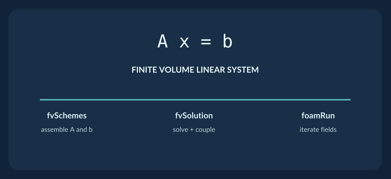
fvSchemes assembles the matrix A and the source b, fvSolution decides how each system is solved and how the equations are coupled, foamRun (with the selected module) iterates the fields in time or until convergence.Prerequisites. This part comes after the initial seven CFD exercises of the course (the seven-step workflow applied in the worked cases, starting with the laminar channel flow and Poiseuille validation) and after Part 5 on numerical schemes. Platform: OpenFOAM Foundation 14.
Before you begin: learning contract
The aim is to read, justify, inspect and modify system/fvSolution without confusing linear solver settings with discretisation, physical models or simulation time control.
What you should be able to do
- Translate a finite-volume equation into the idea of a sparse algebraic system A x = b.
- Locate the linear solver and convergence settings used for
p,Uand optional model fields. - Distinguish
tolerance,relTol,maxIter, outer residual targets and physical convergence. - Explain the purpose of SIMPLE, PIMPLE, pressure correctors and relaxation.
- Use the Foundation v14 User Guide and tutorial files to justify a change.
Version · Version matters
The examples use OpenFOAM Foundation v14, where foamRun loads modules such as incompressibleFluid. Older guides referring to simpleFoam or pimpleFoam require careful version interpretation.
Deep dive · From simpleFoam and pimpleFoam to foamRun: what really changed
Up to version 10 of the Foundation distribution each combination of physics and algorithm had a dedicated executable: simpleFoam for steady incompressible flows with SIMPLE, pisoFoam and pimpleFoam for transient ones. From version 11 these executables were replaced by solver modules loaded by a single program, foamRun; the module is selected in system/controlDict with the entry solver incompressibleFluid; (or with foamRun -solver incompressibleFluid).
The consequence for fvSolution matters: in v14 it is no longer the executable name that says whether the algorithm is SIMPLE or PIMPLE. The same incompressibleFluid module handles both cases: steady behaviour is obtained by declaring ddtSchemes { default steadyState; } in fvSchemes and writing a SIMPLE sub-dictionary in fvSolution, as in the v14 guide’s pitzDailySteady tutorial. The linear-solver entries (solvers), on the other hand, have stayed substantially the same: that is why an old fvSolution is often still readable, but its context (executable, model files, dimension names) must be checked.
foamToC -solvers          # list the solver modules available to foamRun
foamInfo incompressibleFluid
foamDictionary -entry solver -value system/controlDict
Before starting
You should already have a working copy of the reference channel, basic knowledge of 0/U, 0/p (Part 3) and controlDict (Part 4), and the ability to inspect fvSchemes (Part 5). The experiments must be performed on copies, never on the authoritative simulation.
Scope
This unit teaches configuration and interpretation. It does not claim that a low residual proves a physically accurate CFD result. Independent checks of conservation, boundary conditions and mesh effects remain necessary.
1. Case architecture: where fvSolution belongs
OpenFOAM separates the physics, discretisation and linear-algebra steps of a CFD case.
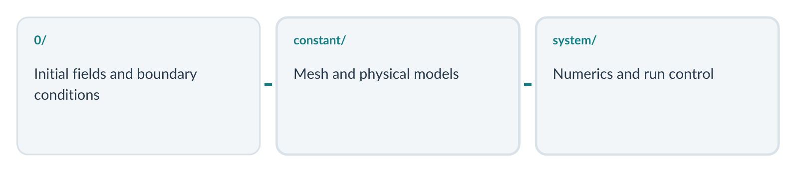
0/ holds initial fields and boundary conditions, constant/ the mesh and physical models, system/ the numerics and run control. fvSolution lives in system/.| File | Controls | Does not control |
|---|---|---|
system/fvSchemes | Approximation of differential operators | The matrix solver type |
system/fvSolution | Linear solvers, tolerances, coupling loops | Mesh dimensions or inlet speed |
system/controlDict | Time, runtime and result writing | Pressure solver preconditioner |
constant/* | Fluid properties and active models | Equation residual tolerances |
0/U, 0/p | Initial/boundary values | SIMPLE iteration counts |
The question this part answers
After the equations have been discretised, which algorithm computes a solution for each field, how accurately is each algebraic system solved, and how do the pressure and velocity updates coordinate with each other?
Important · Vocabulary trap
The word solver has two levels: incompressibleFluid is a fluid solver module; GAMG and smoothSolver are linear algebra solvers configured in fvSolution.
Deep dive · What fvSolution contains and when it is read
According to the v14 User Guide (§4.6), fvSolution contains a solvers sub-dictionary with the linear-solver settings of each equation, a relaxationFactors sub-dictionary and an algorithm-control sub-dictionary, SIMPLE for steady cases or PIMPLE for transient ones. Other modules may read further entries (for instance multiphase modules read phase-fraction-specific controls), but for incompressibleFluid these three blocks are all that is needed.
The file is not read only once. A linear solver’s settings are looked up in the solvers dictionary every time an equation is solved, and with runTimeModifiable active (the usual behaviour, see Part 4) OpenFOAM re-reads the system/ files when they are modified during the run. You can therefore, for example, lower a relaxation factor while the calculation is running; the change takes effect at the next iteration and the log reports the re-reading of the dictionary. It is convenient, but it makes the history of the simulation less reproducible: always record the change and the time at which you made it.
Typical error: if the block for a field that the module must solve is missing, the run stops with a FOAM FATAL IO ERROR of the form “keyword p is undefined in dictionary .../system/fvSolution/solvers”. The message gives both the name being looked up and the dictionary path: it is the first thing to read.
2. Numerical framework: from the PDE to A x = b
Once the numerical schemes have been selected, each discretised equation is assembled into an algebraic system.
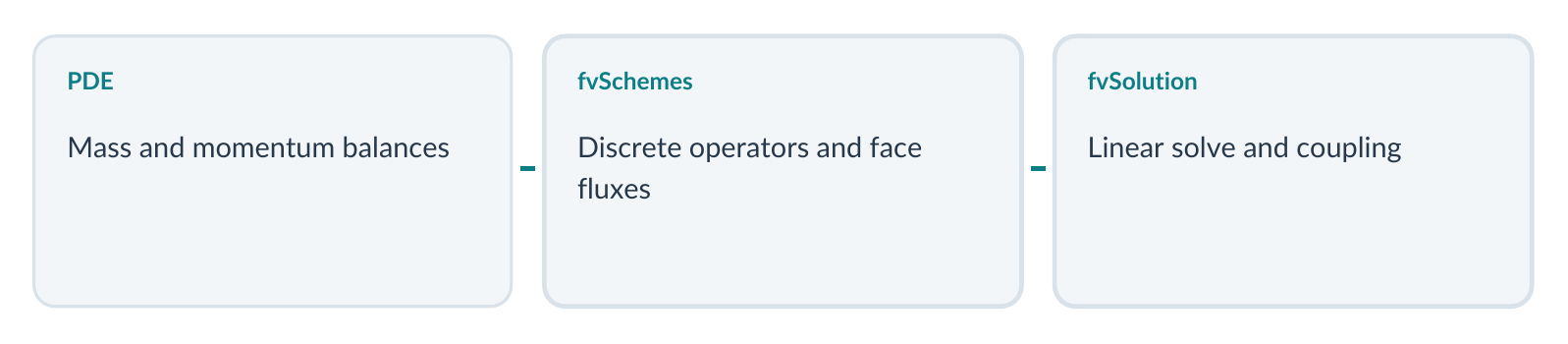
fvSchemes into discrete operators and face fluxes; fvSolution governs the linear solve and the coupling between equations.A schematic finite-volume cell equation
Schematic coefficient equation
aP * phiP + sum(aN * phiN) = bPFor all cells assembled together, the unknown values can be written as a vector x; the coefficients form the typically sparse matrix A, and known contributions form b. Thus A x = b.
A practical incompressible case does not solve every governing equation as one giant fully coupled matrix. The common segregated approach solves equations for one field at a time and uses an outer algorithm to maintain pressure–velocity coupling.
Optional CFD recap · Sparse matrix
A matrix is sparse when most entries are zero. A finite-volume cell interacts mainly with neighbouring cells, so storing and solving the full dense matrix would waste memory and computation.
Deep dive · A worked example: three cells, one 3 × 3 matrix
Consider steady one-dimensional diffusion d/dx(Γ dφ/dx) = 0 on a segment of length 3 divided into three equal cells (Δx = 1, Γ = 1), with φ = 1 at the left boundary and φ = 0 at the right boundary. Integrating over cell P and approximating the diffusive flux through each face by the difference between centres, Γ(φN − φP)/d, gives one equation per cell. For an internal face d = Δx = 1 and the coefficient is 1; for a boundary face the cell centre is d = Δx/2 from the face and the coefficient is 2.
cell 1:  3*phi1 - 1*phi2           = 2   (2 = 2*1, from the left boundary value)
cell 2: -1*phi1 + 2*phi2 - 1*phi3  = 0
cell 3:          -1*phi2 + 3*phi3  = 0   (right boundary value is 0)

    | 3 -1  0 |        | 2 |
A = |-1  2 -1 |    b = | 0 |      x = (5/6, 1/2, 1/6)
    | 0 -1  3 |        | 0 |
The solution, x = (0.833, 0.5, 0.167), coincides with the exact linear profile 1 − x/3 evaluated at the cell centres (0.5, 1.5, 2.5). In the notation used here, aP is the diagonal term (3, 2, 3), the aN are the off-diagonal coefficients (−1) and bP collects the known contributions, here the boundary values. The magnitude of the diagonal is greater than or equal to the sum of the off-diagonal magnitudes in every row: the matrix is diagonally dominant, and it is symmetric because the coefficient linking P to N is the same as the one linking N to P. With one million hexahedral cells the structure is identical: each row has one diagonal entry plus one per internal face of the cell (at most six), so about 7 million non-zeros versus the 1012 entries of a dense matrix.
Deep dive · How OpenFOAM stores the matrix: the LDU format
OpenFOAM does not use a generic sparse format (such as CSR) but the LDU format of the lduMatrix class, built directly on the mesh topology: a diag array with one value per cell, and an upper and a lower array with one value per internal face. Each internal face has an owner cell (lower index) and a neighbour cell: the face’s upper coefficient sits in the owner’s row and the neighbour’s column, the lower coefficient in the transposed position. If the matrix is symmetric, lower is not even allocated.
Boundary faces do not generate off-diagonal entries: the boundary condition (Part 3) contributes an implicit part to the diagonal and an explicit part to the source b. That is why a fixedValue strengthens the diagonal of the adjacent cell (like the 3 in the three-cell example), while a zeroGradient adds nothing. Processor patches in parallel runs (see the worked case on MPI parallel execution) are treated as “interfaces” that exchange values between subdomains at every matrix–vector product: this is why a linear solver’s iteration count can change slightly with the number of processors.
Prediction check
If only div(phi,U) changes in fvSchemes, the assembled matrix may change even when the algorithm and solver entries in fvSolution stay identical. Conversely, changing GAMG to another valid linear solver does not redefine the underlying PDE.
Deep dive · What really changes, in A or in b, when a scheme changes
The “may” in the prediction check is precise. In OpenFOAM many higher-order schemes are implemented as a deferred correction: the implicit part, which goes into the matrix, is that of the upwind scheme, while the difference between the chosen scheme and upwind is computed from the current values and enters the source b. This is the case for linearUpwind: switching from bounded Gauss upwind to bounded Gauss linearUpwind grad(U) leaves the momentum matrix A structurally that of upwind and changes mainly b. Switching instead to Gauss linear (central differencing) changes the interpolation weights and therefore the coefficients of A: diagonal dominance weakens and iterative solvers may need more iterations or become unstable on coarse meshes.
The second statement holds both ways: a different linear solver, if it converges to the same tolerance, produces the same discrete solution apart from the remaining algebraic error. If changing only the linear solver noticeably changes the final result (for example the pressure drop), the tolerances were too loose: it is a useful test to check this.
3. Dictionary structure: inside the solvers dictionary
The first important sub-dictionary maps field names to linear-algebra settings.
Teaching extract: system/fvSolution
solvers
{
    p
    {
        solver          GAMG;
        tolerance       1e-7;
        relTol          0.01;
        smoother        DICGaussSeidel;
    }

    U
    {
        solver          smoothSolver;
        smoother        symGaussSeidel;
        tolerance       1e-5;
        relTol          0.1;
    }
}| Keyword | Interpretation |
|---|---|
p / U | Field whose discrete linear system is solved |
solver | Selected iterative linear-algebra method |
tolerance | Absolute stopping threshold for the residual |
relTol | Required residual reduction relative to the initial value |
smoother | Local iterative operation, required by some methods |
Caution · Example values
The numbers shown illustrate the syntax and a common tutorial pattern; they are not recommended tolerances for every mesh and model.
Deep dive · Every entry a linear-solver block can contain
The table above lists the essential entries. The v14 User Guide documents further ones, with their defaults:
| Entry | Role | Default / notes |
|---|---|---|
solver | Method: PCG, PBiCG, PBiCGStab, smoothSolver, GAMG, diagonal | required |
tolerance | Absolute threshold on the normalised residual | to be specified (the guide lists it as required) |
relTol | Ratio final / initial residual | to be specified (the guide lists it as required) |
maxIter | Maximum number of iterations | 1000 |
preconditioner | For PCG, PBiCG, PBiCGStab | DIC/DILU, FDIC, GAMG, diagonal, none |
smoother | For smoothSolver and GAMG | GaussSeidel, symGaussSeidel, DIC/DILU, DICGaussSeidel |
nSweeps | Smoother sweeps before the residual is recalculated (smoothSolver) | 1 |
The diagonal solver is for explicit equations, whose matrix is diagonal only: it does not iterate and uses no tolerances. To see which names your installation accepts you can deliberately provoke an error on a copy (for example solver xyz;): OpenFOAM replies with the list of valid solvers for that matrix type. To check what the module will actually read after macro expansion, use foamDictionary -expand -entry solvers system/fvSolution.
4. Transient configuration: reading a full v14-style extract
This excerpt follows the structure illustrated in the official v14 description of a transient incompressibleFluid case.
Illustrative v14 tutorial pattern
solvers
{
    p
    {
        solver          GAMG;
        tolerance       1e-7;
        relTol          0.01;
        smoother        DICGaussSeidel;
    }
    pFinal
    {
        $p;
        relTol          0;
    }
    "(U|k|epsilon)"
    {
        solver          smoothSolver;
        smoother        symGaussSeidel;
        tolerance       1e-5;
        relTol          0.1;
    }
    "(U|k|epsilon)Final"
    {
        $U;
        relTol          0;
    }
}
PIMPLE
{
    nNonOrthogonalCorrectors 0;
    nCorrectors              2;
}
Read this as a reusable pattern, not a standalone complete case: the appropriate fields, mesh, properties, schemes and run controls must also exist. The regex group covers turbulence fields only when they are present and used by the selected model.
Deep dive · How OpenFOAM picks the right block: exact names, regex and $ macros
When the module has to solve, for example, the k equation, it looks up the entry k in the solvers dictionary with this precedence: first a key with the exact name; if there is none, the quoted keys that are regular expressions, examined from last to first in file order. The expression must match the whole name: "(U|k|epsilon)" matches k but not kFinal, which is why the second group "(U|k|epsilon)Final" is needed.
The macro $p; copies into the current block all the entries of the p block; entries written after the macro override them (here relTol 0;). $U; also works although there is no literal key U: the macro lookup accepts regex keys, so it finds "(U|k|epsilon)". The expanded result can be checked like this:
foamDictionary -expand -entry solvers/pFinal system/fvSolution
foamDictionary -expand -entry solvers system/fvSolution     # whole block, macros expanded
In the PIMPLE block of this extract nOuterCorrectors does not appear: the default 1 applies, i.e. “PISO” mode (a single outer pass per time step with two pressure corrections), suitable when the Courant number stays below 1. In a laminar case such as the reference channel k and epsilon do not exist: the regex group is harmless but useless, and it is better to reduce it to U and UFinal.
5. Residuals and stopping: three different convergence controls
The settings tolerance, relTol and maxIter govern the stopping of an individual linear solve.
| Criterion | Mathematical idea | Meaning |
|---|---|---|
tolerance | rfinal < T | Stop below a residual threshold |
relTol | rfinal / rinitial < R | Stop after a sufficient relative reduction |
maxIter | N reaches the limit | Stop if the iteration cap is reached |
An iterative linear solver generally stops when any of these conditions is reached. Therefore a solver may stop because the relative reduction target is met while the final residual is still above tolerance.
Keywords in a field solver block
tolerance       1e-7;
relTol          0.01;
// maxIter is optional; consult the v14 defaults
Optional CFD recap · Residual versus physical error
The residual measures the mismatch between the current algebraic solution and the discretised equations (with OpenFOAM-specific normalisation). It does not directly quantify mesh error, modelling error, or deviation from experiment.
In the Foundation v14 User Guide, both tolerance and relTol are specified for linear solver entries; maxIter is optional and has a documented default (1000).
Deep dive · OpenFOAM residual normalisation and why the first residual is often 1
The “raw” residual of a system is the vector b − A x, which has the units of the equation and depends on cell size: its absolute value would mean nothing. OpenFOAM makes it dimensionless by dividing it by a normalisation factor built with the mean value x̄ of the current field:
            sum_cells | b - A x |
r = ---------------------------------------------------
     sum_cells ( | A x - A xbar | + | b - A xbar | ) + small
The denominator measures how far the problem “departs” from a uniform solution. Two practical consequences. First: if the initial field is uniform (x = x̄, like internalField uniform 0), the first term of the denominator vanishes and the second equals the numerator, so the initial residual of the first step is 1: it is not an error, it is the normalisation. Second: the residual is a sum (L1 norm) over all cells divided by a similar sum, so it is an average; small residuals can hide a few cells with large errors, one more reason for the physical checks of the following sections.
On maxIter: if the log shows No Iterations 1000 (or the value you set), the solver reached neither tolerance nor relTol and was stopped by the cap. It is not an error message, but it is almost always the symptom of a problem: ill-conditioned matrix, unsuitable solver, poor mesh quality or a solution that is diverging.
6. Numerical reading: a worked residual calculation
A small numerical calculation is often more useful than memorising the names of solver parameters.
Worked example · Illustrative example
Suppose the initial residual is 2 × 10⁻³; tolerance = 1 × 10⁻⁷ and relTol = 0.01. The relative stop threshold is 2 × 10⁻⁵. The linear iteration can therefore stop on the relative criterion before it reaches 10−7.
| Residual during solve | Relative ratio | Relative criterion reached? |
|---|---|---|
| 2.0 × 10⁻³ | 1.000 | No |
| 8.0 × 10⁻⁴ | 0.400 | No |
| 1.5 × 10⁻⁵ | 0.0075 | Yes |
What changes when relTol = 0?
If relTol = 0, the relative reduction condition is effectively disabled. The solver then continues toward the tolerance threshold, unless it hits another stopping condition such as maxIter.
Check · Question
If you change relTol from 0.1 to 0.01 while keeping the initial residual and all other conditions identical, would you normally expect the linear solve to do more or fewer iterations? Explain before trying. (Worked answer in section 24.)
Deep dive · Estimating the iteration count with a constant reduction factor
Many iterative methods, after the first iterations, reduce the residual by a roughly constant factor ρ per iteration (the convergence factor). In the table the first step takes the residual from 2.0 × 10⁻³ to 8.0 × 10⁻⁴, i.e. ρ ≈ 0.4. If ρ stayed at 0.4, after n iterations the ratio would be 0.4n, and the iterations needed for each criterion can be estimated:
| Criterion | Ratio to reach | Minimum n (ρ = 0.4) |
|---|---|---|
relTol 0.1 | 0.1 | ln 0.1 / ln 0.4 = 2.5 → 3 |
relTol 0.01 | 0.01 | ln 0.01 / ln 0.4 = 5.0 → 6 |
relTol 0, tolerance 1e-7 | 10−7 / 2 × 10−3 = 5 × 10⁻⁵ | ln(5 × 10⁻⁵) / ln 0.4 = 10.8 → 11 |
The estimate shows the general rule: each extra decade of reduction costs about ln 10 / |ln ρ| iterations (here about 2.5). The actual value in the table falls faster (1.5 × 10⁻⁵ corresponds to a ratio of 0.0075), because ρ is not constant: with GAMG in particular each cycle reduces the residual far more than a factor 0.4. The correct way to measure ρ on your own case is to read the initial residual, final residual and iteration count in the log: ρ ≈ (rfinal/rinitial)1/N. With the log lines of section 7: for p, (0.00008/0.014)1/5 ≈ 0.36.
7. Run diagnostics: how to read a solver log
OpenFOAM reports residuals during the calculation. Treat the individual matrix solve separately from the overall CFD convergence history.
Illustrative log lines – not measured output
GAMG:  Solving for p, Initial residual = 0.014,
       Final residual = 0.00008, No Iterations 5

smoothSolver:  Solving for Ux, Initial residual = 0.0032,
Final residual = 0.00021, No Iterations 2| Log item | How to interpret it |
|---|---|
GAMG / smoothSolver | Which linear method handled the equation |
p, Ux | Which field/component was being solved |
Initial residual | Mismatch before this particular solve |
Final residual | Mismatch after this particular solve |
No Iterations | Work performed by this linear solve |
Do not confuse two histories
Inside a solve: a residual falls as one matrix system is iterated. Across time steps or outer iterations: the reported initial residual can change as pressure, velocity and other fields are updated and equations are reassembled.
Check · Physical checks
Even with small reported residuals, also inspect continuity/mass-balance indicators, boundary-condition consistency and the observable that matters to the simulation (e.g. pressure drop).
Deep dive · Anatomy of one time step in a foamRun log
Here is what one step of a 3D transient incompressibleFluid case with PIMPLE in PISO mode (nOuterCorrectors 1, nCorrectors 2) typically looks like. The numbers are illustrative; the structure is what you will find in your log.
Courant Number mean: 0.12 max: 0.45
Time = 0.0025s

smoothSolver:  Solving for Ux, Initial residual = 0.0032, Final residual = 0.00021, No Iterations 2
smoothSolver:  Solving for Uy, Initial residual = 0.0051, Final residual = 0.00030, No Iterations 2
smoothSolver:  Solving for Uz, Initial residual = 0.0047, Final residual = 0.00028, No Iterations 2
GAMG:  Solving for p, Initial residual = 0.014, Final residual = 0.00008, No Iterations 5
time step continuity errors : sum local = 2.1e-07, global = -3.4e-09, cumulative = -3.4e-09
GAMG:  Solving for p, Initial residual = 0.0021, Final residual = 9.1e-08, No Iterations 9
time step continuity errors : sum local = 3.0e-10, global = 1.2e-12, cumulative = -3.4e-09
ExecutionTime = 0.41 s ClockTime = 0 s- The three lines
Ux,Uy,Uzare the momentum predictor: the vector equation is solved component by component with the same matrix. In a 2D case withemptypatches the component normal to the plane is not solved and its line is missing. - The two
plines are the two pressure corrections (nCorrectors 2); the second uses thepFinalsettings (section 8), so it goes down totoleranceand needs more iterations. time step continuity errorsis the mass-balance indicator called for by the “Physical checks” box:sum localis the weighted mean of the absolute flux divergence,globalits signed sum,cumulativethe sum over time. Values that grow step after step indicate that pressure is not solved well enough.- With a preconditioner its name appears as a prefix:
DICPCG: Solving for p,DILUPBiCGStab: Solving for Ux.
Deep dive · Extracting residual histories from the log
To compare two runs (as Lab A requires) you need numbers, not impressions. A few ways, from the simplest to the most structured:
# 1. every pressure solve: initial residual and iteration count
grep "Solving for p" log.foamRun | awk -F'[=,]' '{print $3, $NF}' | head

# 2. total linear iterations for p over the whole run
grep "Solving for p" log.foamRun | awk '{s += $NF} END {print s}'

# 3. continuity errors only
grep "continuity errors" log.foamRun | tail -5

# 4. split the log into one file per quantity (logs/p_0, logs/Ux_0, ...)
foamLog log.foamRun
Alternatively the residuals function writes the initial residuals to a text file during the run: add #includeFunc residuals(p, U) to the functions sub-dictionary of controlDict (Part 4) and you will find the data in postProcessing/residuals/; check its options with foamInfo residuals. Remember that these files record the initial residual of each solve: it is the “across steps” history, not the “inside a solve” one.
8. Efficiency pattern: final solver entries and reuse
A field may be solved several times per time step or outer iteration. The final solve can use a different stopping rule.
Pressure and final pressure solves
p
{
    solver          GAMG;
    tolerance       1e-7;
    relTol          0.01;
    smoother        DICGaussSeidel;
}
pFinal
{
    $p;
    relTol          0;
}pdefines the regular pressure linear-solver configuration.pFinalis a specially named configuration used when the algorithm requests its final pressure solve.$p;reuses the entries ofp; the laterrelTol 0;changes the final relative stopping condition.- This pattern avoids duplicating every parameter and helps keep configurations consistent.
Note · Naming is meaningful
A pFinal dictionary is not another physical field file. Its meaning is determined by the solver algorithm when selecting settings for the final algebraic solve.
The Final pattern is used especially when pressure is corrected several times per step. It lets earlier corrections be less expensive while the last correction is more tightly converged.
Deep dive · When exactly the Final entry is used, and what happens if it is missing
In the Foundation implementation the suffix Final is appended to the field name when the algorithm is in its last iteration: for velocity and the other fields during the last PIMPLE outer loop (with nOuterCorrectors 1, therefore, at every step); for pressure in the last pressure correction of the last outer loop (and, if there are non-orthogonal correctors, in the last of them). The v14 User Guide describes the purpose: solving the equation with separate settings for the final corrector, typically relTol 0, so that each time step converges down to tolerance.
Why it matters in transient cases: the algebraic error left at the end of a step is never corrected again and accumulates over time as continuity error. Intermediate corrections, by contrast, will be superseded by the next one anyway: there is no point paying a high price for them. In the log of section 7 the difference is visible: 5 iterations with relTol 0.01, 9 with relTol 0.
If the entry is missing in a transient case, the run stops at the first final solve with an error of the form “keyword pFinal is undefined in dictionary .../system/fvSolution/solvers”. In steady cases with SIMPLE (like Teaching file A in section 18 and the pitzDailySteady tutorial) Final entries normally do not appear.
9. Shared settings: regular expressions for fields
OpenFOAM dictionary keys can use regular-expression matching to avoid repetition when several field equations require the same solver settings.
Grouped fields
"(U|k|epsilon)"
{
    solver          smoothSolver;
    smoother        symGaussSeidel;
    tolerance       1e-5;
    relTol          0.1;
}

"(U|k|epsilon)Final"
{
    $U;
    relTol          0;
}
The first group can match U, k or epsilon. The second matches the corresponding names ending with Final. When a turbulence model changes, verify that the solver configuration covers its actual fields.
A practical discipline
- Use explicit field names first; add groups once you understand the patterns.
- Avoid overly broad regular expressions that silently catch unrelated fields.
- Inspect the expanded file and tutorial examples before using a newly introduced pattern.
Check · Exercise
Explain why omega is not covered by "(U|k|epsilon)". Modify the pattern to include it without changing the other alternatives. (Solution in section 24.)
Deep dive · Regex key syntax and the fields solved by common models
- Double quotes are required: the quoting is what tells OpenFOAM to treat the key as a regular expression. Without quotes,
(U|k|epsilon)is not even a valid word. - Matching is on the whole name:
"U.*"catchesU,UFinalbut also, for example, anyUa;".*"catches everything and is legitimate only in contexts such asrelaxationFactors(section 19). - The dot is a metacharacter: in quotes,
"alpha.water"also matchesalphaXwater. When the literal dot matters, the safest solution is to write the exact unquoted name (alpha.water), which is compared character by character. - Precedence: the exact name always wins; among several regexes the last one in the file wins. An explicit
Ublock written after the group therefore takes precedence over the group forU.
Which fields must be covered depends on the model in constant/momentumTransport (Part 7):
| Model | Fields with a transport equation |
|---|---|
laminar (reference channel) | none besides U and p |
kEpsilon, realizableKE, RNGkEpsilon | k, epsilon |
kOmega, kOmegaSST | k, omega |
SpalartAllmaras | nuTilda |
nut, the turbulent viscosity, is computed by the model and has no equation of its own: it needs no solvers entry. If a solved field is not covered, the error appears at that field’s first solve, with the message “keyword omega is undefined in dictionary …/solvers”.
10. Choosing solvers: symmetric and asymmetric matrices
Not every linear solver is appropriate for every matrix: the matrix algebra matters.
| Solver | Typical matrix class | Key observation |
|---|---|---|
PCG | Symmetric | Preconditioned conjugate-gradient method |
PBiCG / PBiCGStab | Asymmetric | Bi-conjugate-gradient family |
smoothSolver | Supported classes | Iterative sweeps with a chosen smoother |
GAMG | Common pressure systems | Multilevel algorithm, coarse-grid correction |
The symmetric/asymmetric distinction depends on the assembled operator. Advection terms often introduce asymmetry; diffusion-related operators can lead to symmetric matrices under suitable discretisation and boundary treatment.
Error class · Helpful failure
Choosing PCG for an asymmetric equation can trigger an error listing the valid asymmetric solvers. This is useful diagnostic information, not a reason to change several settings randomly.
Optional CFD recap · Matrix symmetry
A matrix is symmetric if Aij = Aji. The choice of discretised operators and coefficients, not merely the name of the physical field, determines whether the property holds.
Deep dive · Where asymmetry comes from: the three-cell example with convection
Take the three cells of section 2 again and add a convective flux F = 1 towards +x, discretised with upwind: on each cell’s outflow face the transported value is the cell’s own (contribution +F on the diagonal), on the inflow face it is that of the upstream cell (contribution −F on the upstream neighbour’s coefficient). The row of cell 2 becomes (2 + F) φ2 − (1 + F) φ1 − φ3 = 0:
diffusion only            diffusion + upwind convection (F = 1)
| 3 -1  0 |               | 4 -1  0 |
|-1  2 -1 |               |-2  3 -1 |
| 0 -1  3 |               | 0 -2  4 |
symmetric: A12 = A21      asymmetric: A21 = -2, A12 = -1
The momentum equation always contains the convective term div(phi,U), so its matrix is asymmetric; the pressure equation of the SIMPLE/PIMPLE algorithms is instead a Laplace (or Poisson) equation ∇·((1/A)∇p) = ∇·(HbyA), with a symmetric matrix. That is why in the tutorials p uses GAMG or PCG, while U, k, epsilon use smoothSolver or PBiCGStab.
A clarification on the table: the v14 User Guide pairs PCG with symmetric matrices and PBiCG with asymmetric ones, but presents PBiCGStab as a stabilised variant usable for both classes; indeed the foamSearch output shown in the guide includes tutorials that use it for p as well. The table’s “asymmetric” row should be read as “suitable for asymmetric too”. GAMG and smoothSolver accept both classes, provided a compatible smoother is chosen (section 11).
Deep dive · What the compatibility error looks like
According to the v14 guide, using a symmetric solver on an asymmetric matrix (or vice versa) produces a FOAM FATAL IO ERROR. The typical form is the following; the exact list depends on the version and the libraries loaded:
--> FOAM FATAL IO ERROR:
Unknown asymmetric matrix solver PCG

Valid asymmetric matrix solvers are :
(
GAMG
PBiCG
PBiCGStab
smoothSolver
)

file: .../system/fvSolution/solvers/U from line ... to line ...
Read it as the box teaches: the wrong keyword is solver, the file and block are given in the last line, the matrix class (“asymmetric”) is written in the message and the valid alternatives are listed. There is only one fix: change solver (and therefore preconditioner, because DIC is for symmetric matrices only: with PBiCGStab use DILU).
11. Linear algebra controls: smoothers and preconditioners
Some iterative methods use additional settings that improve convergence by transforming the problem or applying inexpensive local iterations.
Preconditioners
A preconditioner transforms the algebraic problem so that the iterative method converges more effectively. Foundation v14 examples include DIC, DILU and FDIC for appropriate matrix structures.
Illustrative asymmetric-solver syntax
U
{
    solver          PBiCGStab;
    preconditioner  DILU;
    tolerance       1e-6;
    relTol          0.05;
}
Smoothers
A smoother reduces high-frequency error components through local iterations. Common choices include GaussSeidel, symGaussSeidel and DICGaussSeidel. The smoothSolver method requires an appropriate smoother setting.
Smooth solver example
U
{
    solver          smoothSolver;
    smoother        symGaussSeidel;
    tolerance       1e-5;
    relTol          0.1;
}
Note · Interpretation
Do not read smoother and preconditioner as interchangeable keywords: their role and acceptable choices depend on the selected linear solver.
Deep dive · What Gauss-Seidel, DIC and DILU actually do
Gauss-Seidel. The cells are visited in order and each is updated by solving its own equation with the latest neighbour values: φP ← (bP − Σ aN φN) / aP. Each update propagates information by one cell only, so errors that oscillate from cell to cell (high frequency) vanish within a few sweeps, while those spread over the whole domain decay very slowly. symGaussSeidel performs a forward and a backward sweep, removing the directional bias tied to cell numbering: it is the preferred smoother in the tutorials for U and turbulence fields. The nSweeps entry (default 1) sets how many sweeps are made before the residual is recalculated.
DIC and DILU. They are incomplete factorisations: an approximation M ≈ A = L D U is built with the same sparsity as A (no fill-in) and in which, in the “diagonal” variant used by OpenFOAM, only the diagonal is modified. Solving with M costs about two substitution sweeps, and the Krylov method works on the preconditioned system M−1A x = M−1b, which is much better conditioned. DIC (incomplete Cholesky) requires a symmetric matrix; DILU (incomplete LU) is the version for asymmetric matrices; FDIC is a faster version of DIC that precomputes reciprocal quantities. The same objects can act as smoothers.
DICGaussSeidel applies DIC smoothing followed by Gauss-Seidel and is the classic choice as the GAMG smoother for pressure: being DIC-based, it is for symmetric matrices (for an asymmetric equation solved with GAMG use GaussSeidel or symGaussSeidel). The v14 guide also lists GAMG itself among the preconditioners (a multigrid cycle preconditioning PCG), diagonal (generally not used) and none.
| Solver | Requires | Example combination |
|---|---|---|
PCG | preconditioner | DIC or FDIC (symmetric) |
PBiCG, PBiCGStab | preconditioner | DILU for U; DIC if used for p |
smoothSolver | smoother | symGaussSeidel or GaussSeidel |
GAMG | smoother | DICGaussSeidel or GaussSeidel for p |
12. Multigrid concept: GAMG, why multiple levels?
Generalised geometric-algebraic multigrid (GAMG) is commonly used for the pressure equation in OpenFOAM tutorials.
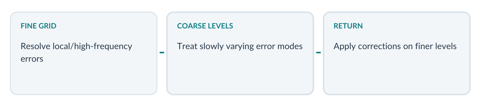
Many iterative methods remove rapidly varying errors quickly but struggle with slowly varying ones. A hierarchy of coarser systems can resolve these long-wavelength components more economically.
GAMG option example
p
{
    solver                GAMG;
    tolerance             1e-7;
    relTol                0.01;
    smoother              DICGaussSeidel;
    nCellsInCoarsestLevel 10;
}
Parameters worth recognising
nCellsInCoarsestLevel: approximate target size of the coarsest level.cacheAgglomeration: reuse agglomeration information where applicable.mergeLevels: multilevel coarsening strategy; changing it can alter robustness and performance.nPreSweeps/nPostSweeps: smoothing work on different levels.
Workflow · Do not over-tune early
For a first experiment, retain the existing GAMG options and change one controlled parameter only after recording a baseline. A change that reduces iteration count is not automatically a physically better solution.
Deep dive · Why multigrid works: error frequencies and cost per cell
Decompose the error e = x − xexact into Fourier modes. A Gauss-Seidel iteration strongly damps modes whose wavelength is a few cells, but a mode spread over n cells is reduced only by a factor of about 1 − c/n2 per sweep: on a mesh of 200 cells per side tens of thousands of sweeps would be needed. The idea of multigrid is that an error that is smooth on the fine grid becomes oscillatory on a coarser grid: after a few smoothing sweeps (pre-sweeps) the residual is transferred to a level with fewer cells, where the same smoother is effective again; going down to the coarsest level (about nCellsInCoarsestLevel cells) the system is so small it is solved almost exactly; the correction is then interpolated upwards and refined with further sweeps (post-sweeps). The result is a cycle count almost independent of mesh size and a cost proportional to the number of cells.
Comparison with PCG: the conjugate-gradient iteration count grows as the square root of the condition number, which for a Laplacian grows as (L/h)2; halving the cell size therefore roughly doubles the PCG iterations, while those of GAMG stay almost the same. That is why GAMG dominates for pressure on medium-to-large meshes, whereas on small meshes (such as the teaching channel with a few thousand cells) the difference is minimal. “Algebraic” means that the coarse levels are not geometrically built meshes but cell agglomerations decided from the matrix coefficients (in the tutorials with the faceAreaPair agglomerator, which pairs cells across their largest faces).
Deep dive · The GAMG options documented in v14 and their defaults
| Option | Default | Meaning |
|---|---|---|
smoother | required | Smoother used on every level |
agglomerator | faceAreaPair (in tutorials) | Cell agglomeration method |
cacheAgglomeration | true | Keeps the hierarchy between solves (a static mesh does not change) |
nCellsInCoarsestLevel | 10 | Target size of the coarsest level |
directSolveCoarsest | false | Direct rather than iterative solve on the coarsest level |
mergeLevels | 1 | How many agglomeration levels to merge in one step (1 = gradual coarsening) |
nPreSweeps | 0 | Sweeps before moving down to the coarser level |
preSweepsLevelMultiplier / maxPreSweeps | 1 / 4 | Growth and cap of pre-sweeps with level |
nPostSweeps | 2 | Sweeps after returning from the coarser level |
postSweepsLevelMultiplier / maxPostSweeps | 1 / 4 | Growth and cap of post-sweeps |
nFinestSweeps | 2 | Sweeps on the finest level |
A note on reading the guide: the v14 User Guide writes this entry as directSolveCoarset; the name used in the code and in dictionaries is directSolveCoarsest, but before using it check its spelling in the tutorials with foamSearch. For the first experiment the advice of the box still holds: these defaults are fine in the vast majority of cases.
13. Relaxation factors: under-relaxation for stability
Under-relaxation limits changes from one nonlinear/segregated iteration to the next and is particularly important for steady-state calculations.
Steady-state style example
relaxationFactors
{
    fields
    {
        p               0.3;
    }
    equations
    {
        U               0.7;
    }
}| Location | What is relaxed |
|---|---|
fields | The field after the linear system is solved |
equations | The algebraic equation before solution |
Relaxation below 1 generally makes changes more conservative. This can improve stability, but may also slow progress. The best factor depends on mesh quality, coupling algorithm, physical model and equation behaviour.
Optional CFD recap · Optional formula
For field relaxation, the idea is φnew = φold + α (φcandidate − φold). With α = 0.3, only 30% of the proposed field update is accepted. Equation relaxation acts on matrix coefficients rather than by directly applying this field blend.
Caution · Steady versus transient
The v14 User Guide discusses under-relaxation for steady cases and notes that, for transient incompressibleFluid cases, equation factors of 1 may be used instead; do not transplant steady-case relaxation values uncritically.
Deep dive · Equation relaxation in formulas, and why 1 does not mean “no effect”
Implicit equation relaxation (Patankar style) divides the diagonal by α and adds to the source a term containing the previous value:
(aP/alpha) * phiP + sum(aN * phiN) = bP + ((1 - alpha)/alpha) * aP * phiP_oldAt convergence φP = φP,old and the two added terms cancel: the final solution is the same, only the path changes. With α = 0.7 the diagonal grows by 1/0.7 ≈ 1.43 times: the matrix becomes more diagonally dominant (iterative solvers converge better) and each iteration takes a shorter step. In OpenFOAM, before α is applied, the diagonal is also raised to at least the sum of the magnitudes of the off-diagonal coefficients: that is why the v14 guide indicates for transient cases a factor 1 for all equations (equations { ".*" 1; }, as in Teaching file B), which slows nothing down but ensures what the guide calls “diagonal equality”, generally required for the convergence of a matrix equation.
Field example. If in a cell pold = 10 m²/s² and the pressure equation proposes pcandidate = 20 m²/s², with α = 0.3 the accepted value is 10 + 0.3 × 10 = 13 m²/s². Indications from the v14 guide: steady tutorials use 0.3 for p and 0.7 for U and for turbulence fields (grouped with a regex); values as high as 0.9 can be stable in some cases, while values well below 0.2 make convergence prohibitively slow. A field or equation absent from relaxationFactors is not relaxed.
14. Pressure–velocity algorithm: SIMPLE, steady-state coupling
SIMPLE links pressure and velocity while seeking a stationary solution of the coupled conservation equations.
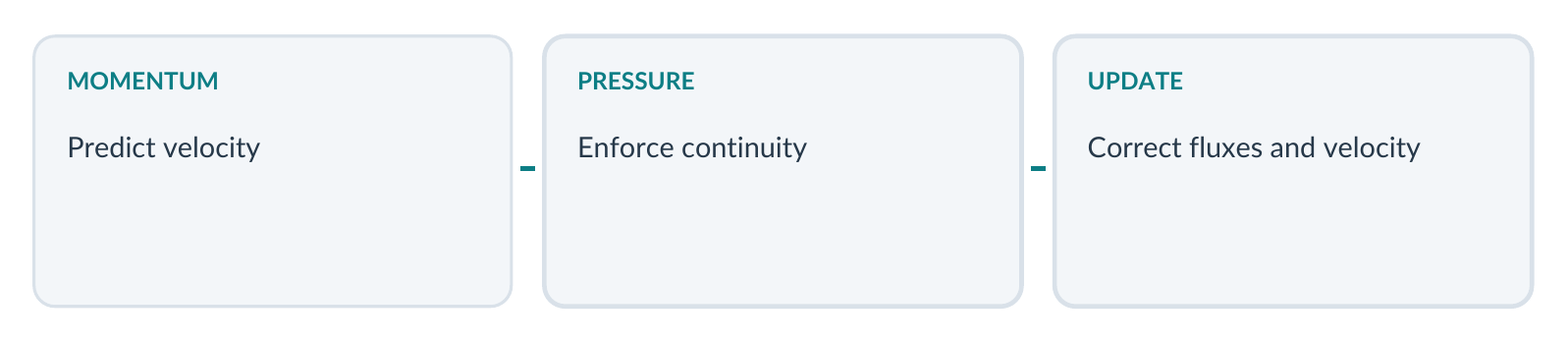
The process repeats across iterations until the required convergence criteria or stopping condition are met. It is not equivalent to solving a single pressure matrix once.
Minimal teaching pattern – steady case
SIMPLE
{
    nNonOrthogonalCorrectors 0;
    residualControl
    {
        p               1e-5;
        U               1e-6;
    }
}
Algorithm settings versus linear tolerance
solvers/p/tolerancegoverns an individual matrix solve.SIMPLE/residualControlspecifies convergence checks for the overall steady iteration, using the applicable field residual measure.nNonOrthogonalCorrectorscontrols additional pressure-equation corrections associated with non-orthogonal discretisation.
Version 14 example · SIMPLEC caution
A tutorial using consistent yes; enables a SIMPLEC-type formulation with relaxation choices that may be carefully tuned. Do not copy such coefficients into ordinary SIMPLE cases without understanding their role.
Deep dive · The SIMPLE steps in formulas
Write the discrete momentum equation of each cell separating the diagonal A from the rest: A UP = H(U) − ∇p, where H collects the neighbour contributions and sources. Hence U = HbyA − (1/A)∇p, with HbyA = H/A. Imposing continuity ∇·U = 0 gives the pressure equation. One SIMPLE iteration of incompressibleFluid proceeds as follows:
- Momentum predictor: the U equation is assembled with the current pressure, relaxed (factor
equations/U) and solved with thesolvers/Usettings (linesUx,Uy,Uzin the log). - Pressure equation: ∇·((1/A)∇p) = ∇·(HbyA), solved with
solvers/p, repeatednNonOrthogonalCorrectorsmore times if requested. - Flux correction: the face flux
phiis corrected with the pressure gradient just computed, and becomes conservative up to the pressure tolerance. - Pressure relaxation (factor
fields/p, e.g. 0.3) and velocity correction U = HbyA − (1/A)∇p. - Model equations (turbulence etc.), then the next iteration.
In the SIMPLEC formulation (consistent yes;) 1/(A − ΣH1) is used instead of 1/A, where ΣH1 is the sum of the neighbour coefficients: the response of the neighbouring cells is approximately accounted for, the pressure correction is more “consistent” and pressure relaxation becomes largely unnecessary. The v14 guide warns, however, that in the pitzDailySteady tutorial SIMPLEC convergence is very sensitive to the relaxation factors, which there are 0.9 and carefully tuned: they are not suitable for standard SIMPLE, and SIMPLEC is generally reliable only on simple geometries.
Deep dive · How residualControl works and what it writes in the log
At the start of each steady iteration the module compares the initial residual of the first solve of each field listed in residualControl with the given threshold (for a vector such as U the solved components are considered). When all listed fields are below threshold, the simulation writes the results and ends before endTime, with a message such as SIMPLE solution converged in 285 iterations (the number reported by the v14 guide for pitzDailySteady). Fields not listed are not checked. If the thresholds are never reached, the run continues up to the controlDict endTime (Part 4), where in steady cases “time” is only an iteration counter.
Mind the consistency between the two levels: the initial residual of an iteration cannot drop much below the reduction that the linear solver achieves at each iteration. With tolerance 1e-7 for p and residualControl p 1e-5 the combination is sensible; with a linear tolerance looser than the residualControl threshold, the threshold might never be reached.
15. Inner and outer loops: PIMPLE, transient coupling
PIMPLE combines pressure–velocity correction with optional repetition of the coupled system within a time step.
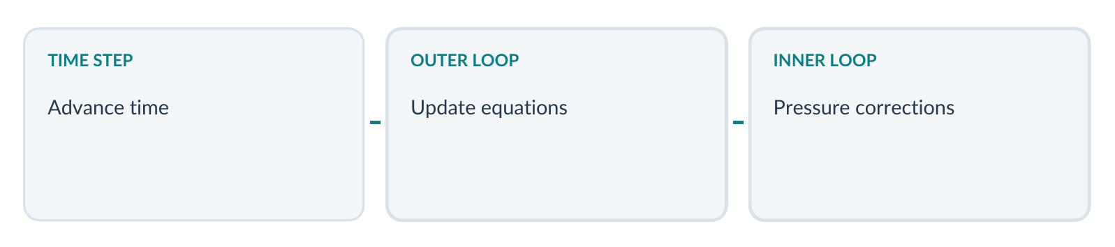
PIMPLE control entries
PIMPLE
{
    nOuterCorrectors         1;
    nCorrectors              2;
    nNonOrthogonalCorrectors 0;
    momentumPredictor        yes;
}| Parameter | What it controls |
|---|---|
nOuterCorrectors | Repetitions of the coupled equation system per step |
nCorrectors | Pressure/velocity corrections within the step |
nNonOrthogonalCorrectors | Additional pressure corrections for non-orthogonal contribution |
momentumPredictor | Whether an initial momentum predictor is solved |
Important · Loop counts are not linear iterations
A pressure solve performed twice by PIMPLE is not the same as a linear solver performing two iterations inside one pressure solve. These nested levels must remain conceptually separate.
Deep dive · PISO mode, outer loops and the momentum predictor
With nOuterCorrectors 1 PIMPLE reduces to the PISO algorithm: one momentum predictor and nCorrectors pressure corrections per step, without reassembling the momentum equation. It is accurate and cheap if the maximum Courant number stays roughly below 1 (see the deltaT control in Part 4). According to the v14 guide nCorrectors is typically 2 or 3 and nOuterCorrectors typically 1.
With nOuterCorrectors > 1 the whole system is reassembled and solved several times within the same step: the non-linearities (the convective flux phi appearing in the U matrix) are updated, and time steps with a Courant number well above 1 become possible. In this regime the outer iterations behave like mini steady iterations and relaxation may be needed even in transient runs. To avoid wasting outer loops when the step has already converged, the Foundation implementation provides an outerCorrectorResidualControl sub-dictionary (per-field thresholds that end the outer loops early): before using it, look for an example in the tutorials with grep -r outerCorrectorResidualControl $FOAM_TUTORIALS.
momentumPredictor no; skips the solution of the momentum equation and goes straight to pressure, using the previous step’s velocity to build HbyA. The v14 guide indicates it can be switched off for some flows, for example at low Reynolds number and multiphase. The consequence is immediately visible in the log: the Solving for Ux/Uy/Uz lines disappear.
16. Stopping criteria: three nested iteration levels
One of the most common mistakes is to interpret every occurrence of the word iteration as the same numerical process.
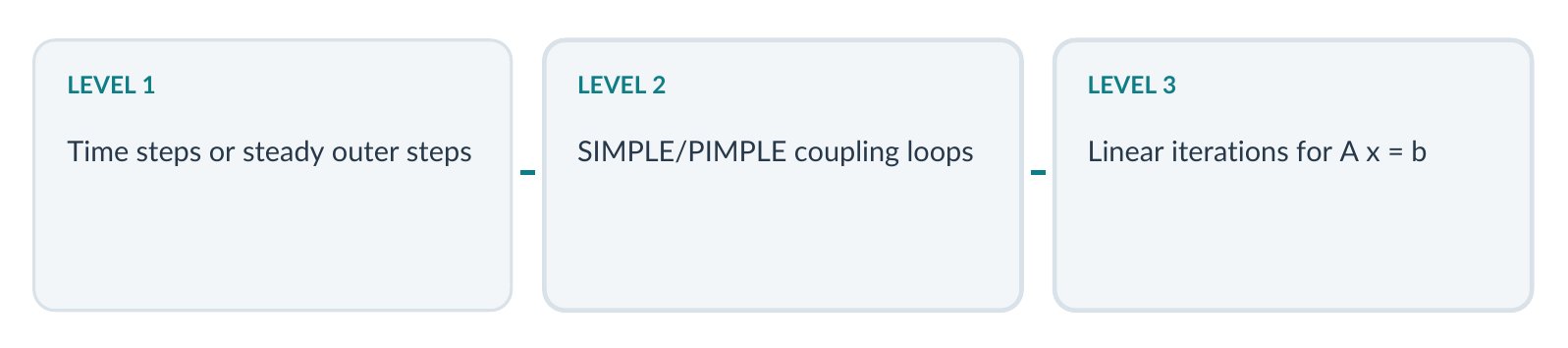
Three different observations
| Observation | Driven by |
|---|---|
| Simulation time, write events | controlDict |
| Number of pressure correction passes | SIMPLE/PIMPLE entries in fvSolution |
| Iterations to reduce p or U residual | solvers/p and solvers/U in fvSolution |
If a run is expensive, identify which loop consumes work before changing parameters. More outer correctors may increase the number of systems assembled and solved; a tighter relTol may increase iterations inside each linear solve.
Think through · Worked scenario
A transient step may perform 2 pressure corrections; the first pressure matrix solve may require 4 GAMG iterations and the final pressure matrix solve 7. These are two different iteration counts, each describing a different level of the algorithm.
Deep dive · Counting the work of one step: a worked example
Take a PIMPLE step with nOuterCorrectors 2, nCorrectors 2, nNonOrthogonalCorrectors 1 and momentumPredictor yes, in 3D. The number of linear systems solved is:
| Equation | Count | Settings used |
|---|---|---|
| Momentum | 2 outer loops × 3 components = 6 | U in the first loop, UFinal in the second |
| Pressure | 2 outer × 2 correctors × (1 + 1) non-orthogonal = 8 | p for 7 solves, pFinal for the last one |
If each p solve costs on average 5 GAMG iterations and the final one 12, the step needs about 7 × 5 + 12 = 47 GAMG cycles; setting nOuterCorrectors to 1 brings the pressure solves down to 4 and roughly halves the work, whereas tightening the p relTol from 0.01 to 0.001 would keep 8 solves but make each longer. They are two different levers on two different levels: to know which to use you must first read in the log which level weighs most (section 7).
17. Geometry–algorithm link: mesh quality and pressure reference
Discretisation correction, mesh non-orthogonality and pressure reference are numerically separate issues.
Non-orthogonal correction
Non-orthogonal meshes can require explicitly treated corrections in the pressure-equation Laplacian. The setting nNonOrthogonalCorrectors repeats the pressure solution to update these contributions, but it does not repair a badly designed mesh.
Illustrative configuration
PIMPLE
{
    nCorrectors              2;
    nNonOrthogonalCorrectors 1;
}
Deep dive · Where the non-orthogonal correction comes from and when it is needed
The diffusive flux through a face requires the face-normal gradient, (∇p)f · Sf. On an orthogonal mesh the vector d joining the two cell centres is parallel to the normal Sf and the gradient is obtained exactly from the difference (pN − pP)/|d|, an implicit part that enters the matrix. If d and Sf form an angle θ (the non-orthogonality), Sf is split as Δ + k with Δ parallel to d: the Δ part stays implicit, the k · (∇p)f part must be computed from the gradient of the current solution and enters b as an explicit correction. Each non-orthogonal corrector solves the pressure equation again with the updated gradient.
On a single-block blockMesh mesh such as the channel of Part 2 θ = 0 everywhere and no correctors are needed: 0 is the right choice. checkMesh reports Mesh non-orthogonality Max: … average: … and flags faces beyond 70° as severely non-orthogonal. The v14 guide indicates typical values of 0 for steady cases and 1 for transient ones; on highly distorted meshes 1–2 correctors are combined with limited Laplacian schemes (Gauss linear limited corrected 0.33, Part 5). In steady cases the non-orthogonality is in any case “absorbed” by the subsequent SIMPLE iterations, which is why 0 is enough there.
Pressure reference
In a closed incompressible domain with no prescribed absolute pressure level, pressure can be determined only up to an additive constant. A reference cell and reference value remove this indeterminacy.
Inside SIMPLE or PIMPLE when needed
pRefCell        0;
pRefValue       0;
Caution · When not needed
A case with an adequate fixed pressure reference at a boundary may not require the same internal referencing. Determine this from the actual pressure boundary conditions and module behaviour, not from a generic template.
Optional CFD recap · Pressure gauge
In many incompressible-flow formulations, the pressure gradients drive velocity. Adding a constant to pressure does not change those gradients; a reference fixes the arbitrary level in a closed system.
Deep dive · pRefCell and pRefValue in practice
- The entries are read only if the pressure field needs a reference, i.e. if no patch imposes a value (no
fixedValueor equivalent type). In the reference channel, withfixedValue0 at the outlet (Part 3), they would be ignored even if present. pRefCellis the index of a cell (0 is the first cell of the mesh numbering),pRefValuethe pressure value assigned there, in the units of thepfield (m²/s² forincompressibleFluid). The v14 guide usually places them in theSIMPLEorPIMPLEsub-dictionary.- The classic example is the lid-driven cavity: walls only,
zeroGradientforpeverywhere, hencepRefCell 0; pRefValue 0;. - If they are needed and missing, the module stops with an error reporting the absence of the
pRefCellentry (orpRefPoint, the alternative giving a location instead of an index) in the algorithm dictionary. Without any reference the pressure matrix would be singular: the level ofpwould drift and the linear solver would struggle to converge.
18. Reference file A: a complete steady-style fvSolution
Illustrative configuration for a simple steady incompressibleFluid case with fields p and U. The surrounding case must be physically and numerically compatible.
Teaching file A: system/fvSolution
FoamFile
{
    format          ascii;
    class           dictionary;
    location        "system";
    object          fvSolution;
}

solvers
{
    p
    {
        solver          GAMG;
        tolerance       1e-7;
        relTol          0.01;
        smoother        DICGaussSeidel;
    }
    U
    {
        solver          smoothSolver;
        smoother        symGaussSeidel;
        tolerance       1e-6;
        relTol          0.1;
    }
}
SIMPLE
{
    nNonOrthogonalCorrectors 0;
    residualControl
    {
        p               1e-5;
        U               1e-6;
    }
}
relaxationFactors
{
    fields    { p 0.3; }
    equations { U 0.7; }
}
The values are chosen for explaining dictionary roles; they are not validated optimum settings. For a laminar training case with steadyState in fvSchemes, adapt this file to match the actual solver configuration.
Deep dive · Reading File A line by line and adapting it to the laminar channel
- Header.
version 2.0;is missing, which is optional in v14;class dictionaryandobject fvSolutionmust match the file. solvers. OnlypandU: exactly what alaminarcase needs, with no turbulence fields. No Final entries, because withSIMPLEthey are not needed.SIMPLE. Orthogonal mesh → 0 correctors; nopRefCellbecause the outlet fixes the pressure;residualControlwith fairly strict thresholds (1e-5 forp, 1e-6 forU, the latter equal to the lineartoleranceofU). If the thresholds are not reached, the run goes on toendTime: a situation to recognise in the log, not necessarily an error.relaxationFactors. The compact one-line form (fields { p 0.3; }) is syntactically identical to the multi-line form of section 13.
Before using it on the channel check the nature of the case: foamDictionary -entry ddtSchemes/default -value system/fvSchemes must return steadyState. If it returns Euler or backward, the case is transient and File B of the next section is needed. Also check constant/momentumTransport: with simulationType laminar; File A is complete as it is.
19. Reference file B: a complete transient-style fvSolution
A separate PIMPLE example, including final pressure/velocity solver entries. Do not mix this indiscriminately with the steady case.
Teaching file B: system/fvSolution
FoamFile
{
    format          ascii;
    class           dictionary;
    location        "system";
    object          fvSolution;
}
solvers
{
    p
    {
        solver          GAMG;
        tolerance       1e-7;
        relTol          0.01;
        smoother        DICGaussSeidel;
    }
    pFinal
    {
        $p;
        relTol          0;
    }
    U
    {
        solver          smoothSolver;
        smoother        symGaussSeidel;
        tolerance       1e-6;
        relTol          0.1;
    }
    UFinal
    {
        $U;
        relTol          0;
    }
}
PIMPLE
{
    nOuterCorrectors         1;
    nCorrectors              2;
    nNonOrthogonalCorrectors 0;
}
relaxationFactors
{
    equations { ".*" 1; }
}
Deep dive · File A and File B compared
| Item | File A (steady) | File B (transient) | Why |
|---|---|---|---|
Expected ddtSchemes | steadyState | Euler or backward | The time scheme decides which algorithm makes sense |
| Algorithm | SIMPLE | PIMPLE | Iteration towards steady state versus time marching |
| Final entries | absent | pFinal, UFinal | Only in transient runs must the last correction close the step down to tolerance |
| Relaxation | p 0.3 (field), U 0.7 (equation) | ".*" 1 on equations | In transient runs the time term already stabilises; 1 ensures diagonal equality |
| Stopping | residualControl or endTime | endTime | The transient run must cover the physical time interval |
Mixing the two files produces typical errors: a SIMPLE dictionary in a case with Euler is not read as the transient algorithm; a transient case without pFinal stops at the last correction of the first step; 0.3/0.7 relaxation in a transient case with nOuterCorrectors 1 makes each time step inconsistent, because the end-of-step solution no longer satisfies the equations. In File B momentumPredictor does not appear: the default applies, i.e. the predictor is solved.
20. Foundation v14 workflow: inspect fvSolution using CLI tools
The Foundation v14 case-management tools allow targeted inspection instead of manual scrolling through large dictionaries.
Read-only inspection commands
foamDictionary system/fvSolution
foamDictionary -entry solvers system/fvSolution
foamDictionary -entry 'solvers/p/solver' \
    -value system/fvSolution
foamDictionary -entry 'solvers/p/relTol' \
    -value system/fvSolution
The exact ordering shown here follows the Foundation v14 User Guide. Run these commands from the root of the case and compare them with the original file.
Find solver types used in tutorials
foamSearch -c "$FOAM_TUTORIALS" fvSolution \
    solvers/p/solver
Safe editing
Inspect first, make a separate working copy, then edit only the intended parameter. Afterward, inspect the resulting entry again. Keeping a baseline makes the numerical comparison interpretable.
Safety · Caution about destructive utilities
This exercise does not require foamCleanCase or foamListTimes -rm. Those utilities can delete generated mesh/results. Avoid them on the original simulation or research case.
Deep dive · What to expect from these commands, and how to edit traceably
On Teaching file A the two -value queries return the value only, without semicolon: GAMG and 0.01. Without -value you get the full entry (solver GAMG;). Other useful forms, all documented in §4.7 of the v14 guide:
foamDictionary -entry solvers -keywords system/fvSolution   # p, U (or p, pFinal, "(U|k|epsilon)", ...)
foamDictionary -expand system/fvSolution                   # macros such as $p expanded
foamDictionary -entry solvers/p/relTol -set 0.001 system/fvSolution   # edit ONLY on a copy
diff -u ../step06_steady/system/fvSolution system/fvSolution          # record exactly what changed
foamSearch -c counts how many times each value of the searched entry appears in all files with that name below the given directory. The v14 guide shows as an example 64 occurrences of GAMG, 26 of PCG, 5 of smoothSolver and 2 of PBiCGStab for solvers/p/solver: the numbers in your installation may differ, but the indication remains that GAMG is the most common choice for pressure. The same technique works for any entry, for example foamSearch -c "$FOAM_TUTORIALS" fvSolution SIMPLE/consistent to find out which tutorials use SIMPLEC.
21. Guided practical — Lab A: controlled solver experiment
Experiment on an isolated clone of a Foundation v14 tutorial, such as pitzDailySteady, after confirming its actual directory location.
1. Make a separate case copy
Working copy only
mkdir -p "$HOME/OpenFOAM/training_step06"
cp -a "$FOAM_TUTORIALS/modules/incompressibleFluid/pitzDailySteady" \
   "$HOME/OpenFOAM/training_step06/step06_steady"
cd "$HOME/OpenFOAM/training_step06/step06_steady"
If the distribution places the tutorial elsewhere, find it under $FOAM_TUTORIALS before copying. Do not overwrite an existing step06_steady directory.
Caution · The tutorial path in the v14 guide
The v14 User Guide (§2.1) copies the tutorial from $FOAM_TUTORIALS/incompressibleFluid/pitzDailySteady, that is without the modules/ subdirectory used in the command above. Before copying, check with find "$FOAM_TUTORIALS" -type d -name pitzDailySteady and use the path that the command returns.
2. Inspect and prepare
Do not change any parameter yet
foamVersion
foamDictionary -entry solvers system/fvSolution
foamDictionary -entry SIMPLE system/fvSolution
blockMesh
checkMesh
3. Capture a baseline
Run the case with foamRun and save the terminal log. Record the field solver type, typical initial/final residuals, linear iteration counts and convergence information. Keep the log and original fvSolution for comparison.
4. Change one parameter
On another clone from the same pristine tutorial, change only the relative tolerance for a solver entry that is actually present. Keep mesh, schemes, physical model and run control identical. Compare solver iteration counts and global residual histories.
Deliverable
Baseline/modified solver comparison and one justified conclusion. No claim of improved physical accuracy.
Deep dive · Lab A step by step, with the commands
A possible complete sequence for steps 3 and 4, with the tutorial path of the v14 guide (adapt it to the one found with find). The name step06_relTol for the second clone is an arbitrary choice.
# --- step 3: baseline
cd "$HOME/OpenFOAM/training_step06/step06_steady"
foamRun > log.foamRun 2>&1
grep "solution converged" log.foamRun            # iterations to residualControl, if reached
grep -c "Solving for p" log.foamRun              # number of pressure solves
grep "Solving for p" log.foamRun | awk '{s += $NF} END {print s}'   # total p iterations
foamDictionary -entry solvers/p/relTol -value system/fvSolution     # note the current value

# --- step 4: second pristine clone, one change only
test -e "$HOME/OpenFOAM/training_step06/step06_relTol" && echo "exists: choose another name"
cp -a "$FOAM_TUTORIALS/incompressibleFluid/pitzDailySteady" \
   "$HOME/OpenFOAM/training_step06/step06_relTol"
cd "$HOME/OpenFOAM/training_step06/step06_relTol"
foamDictionary -entry solvers/p/relTol -set 0.01 system/fvSolution  # choose a value different from the baseline
diff -u ../step06_steady/system/fvSolution system/fvSolution        # must show ONE changed line
blockMesh > log.blockMesh 2>&1
foamRun > log.foamRun 2>&1
Collect the results in a table with three comparison rows (SIMPLE iterations to convergence, total p linear iterations, final ExecutionTime) and, separately, a physical control quantity, for example the pressure difference between inlet and outlet. A justified conclusion has the form: “with a tighter relTol each p solve needs on average N more iterations, the number of SIMPLE iterations changes by M and the control quantity varies by less than X%: the cost increases without an appreciable change in the solution”. Note that in steady cases a tighter relTol may even reduce the number of outer iterations: this is exactly the kind of effect the comparison must measure, not assume.
22. Guided debugging — Lab B: diagnose configuration errors
Use intentionally flawed excerpts to learn to identify errors before touching the run.
Example 1: incomplete solver dictionary
Spot the missing keyword
p
{
    solver          GAMG;
    tolerance       1e-7;
    smoother        DICGaussSeidel;
}
Question: what stopping parameter required by the v14 User Guide is missing in this minimal p configuration?
Example 2: wrong matrix solver
Investigate matrix compatibility
U
{
    solver          PCG;
    preconditioner  DIC;
    tolerance       1e-6;
    relTol          0;
}
Question: if the assembled U matrix is asymmetric because of convection, what class of diagnostic could appear? Which family of methods should you investigate?
Method · Do not guess from one log line
Read the first meaningful error, identify its file and keyword, check the matrix/field/model context, and consult the v14 documentation before changing configuration.
Deep dive · Reading the first meaningful error, and an error that does not show itself
OpenFOAM fatal errors always have the same structure: a line --> FOAM FATAL ERROR or FOAM FATAL IO ERROR, the message, then the file with the lines involved and the function that raised the error. To isolate it in a long log:
grep -n "FOAM FATAL" log.foamRun
grep -n -A 15 "FOAM FATAL" log.foamRun | head -40
Example 2 produces an explicit fatal error (section 10) at the first U solve, so it is easy to diagnose. Example 1 is more insidious: the v14 User Guide lists tolerance and relTol as required, but depending on the implementation an omitted entry may not be reported at all and may silently take a default value (for relTol, zero, i.e. no relative criterion). In that case every p solve would run down to tolerance and the only symptom would be a higher-than-expected iteration count in the log. That is why the correct check is not “does the case start?” but reading the expanded dictionary with foamDictionary -expand -entry solvers/p system/fvSolution and comparing it with the documentation.
23. Assessment: independent exercise and capstone
You should now be able to explain a simple fvSolution and make an evidence-based modification.
Independent tasks
- Locate a steady and a transient
incompressibleFluidtutorial in the installed Foundation v14 distribution. - Extract the
solversblocks; list every named field and solver method. - Identify whether the algorithm uses SIMPLE or PIMPLE and the controls of that algorithm.
- Explain any Final entries and regex groups.
- Record any pressure reference values, non-orthogonal correctors and relaxation factors.
- Describe one parameter change, why it might affect linear-solver work, and how to check the prediction empirically.
Deep dive · A working outline for the independent tasks
The following commands carry out the data-gathering part without modifying anything. pitzDailySteady (steady) and pitzDaily (transient) are the natural pair, both cited by the v14 guide; the path must be confirmed as in Lab A.
ls "$FOAM_TUTORIALS/incompressibleFluid"
for c in pitzDailySteady pitzDaily; do
    f="$FOAM_TUTORIALS/incompressibleFluid/$c/system/fvSolution"
    echo "== $c"
    foamDictionary -entry solvers -keywords "$f"
    foamDictionary -entry ddtSchemes/default -value "${f%fvSolution}fvSchemes"
    foamDictionary -entry SIMPLE "$f" 2>/dev/null || foamDictionary -entry PIMPLE "$f"
    foamDictionary -entry relaxationFactors "$f"
done
For each tutorial fill in a sheet with: the list of blocks in solvers and, for each, solver, preconditioner/smoother, tolerance, relTol; which actual names the regexes cover (comparing them with the model in constant/momentumTransport); algorithm and controls (nCorrectors, nOuterCorrectors, nNonOrthogonalCorrectors, consistent, residualControl, pRefCell/pRefValue); relaxation factors. For the last task use the form “change → level affected (section 16) → predicted effect on iterations → how I measure it in the log (section 7)”.
Evidence of learning
| Question | Minimum acceptable answer |
|---|---|
Why fvSolution? | Controls algebraic solves and coupling algorithm |
What is GAMG? | A linear-algebra multigrid solver; not a fluid module |
What does relTol do? | A relative linear residual-reduction threshold |
What is pFinal? | Settings for a final pressure solve when used by the algorithm |
| What is relaxation? | Limits an update/equation change to improve robustness |
| What makes a run valid? | More than low residuals: also physics, conservation and verification |
Pass condition · Completion criterion
You can inspect an unfamiliar fvSolution, identify its field solvers and coupling controls, explain the expected effect of one change, then validate that prediction on a safe copy.
24. Answers to the reasoning exercises
Try the exercises before reading the answers.
Residual-ratio problem
Initial residual = 0.002; relTol = 0.01 allows stopping when the residual decreases below 0.00002. In the example, 0.000015 meets that relative criterion although it is above the 0.0000001 absolute tolerance. Setting relTol = 0 removes this relative shortcut.
Tightening relTol
Reducing relTol from 0.1 to 0.01 requires a greater fractional decrease before the relative criterion is satisfied; all else equal, one would generally expect more linear iterations. The actual count depends on whether the absolute criterion or iteration cap is reached first.
With the reduction factor ρ ≈ 0.4 of section 6, going from 0.1 to 0.01 takes the estimate from 3 to 6 iterations: one more decade of reduction costs about ln 10 / |ln ρ| ≈ 2.5 iterations.
Regex field grouping
"(U|k|epsilon)" does not match omega: the expression lists three exact alternatives and must match the whole name. One possible revised pattern is "(U|k|epsilon|omega)" (and, consistently, "(U|k|epsilon|omega)Final"). Check which fields actually exist before inserting the change.
Missing configuration
In the deliberately incomplete p entry, relTol is missing. According to the v14 linear solver description, tolerance and relTol should both be provided.
Asymmetric matrix
A symmetric-only method such as PCG cannot be applied to an asymmetric matrix. Investigate methods such as PBiCGStab, PBiCG, smoothSolver or an appropriate GAMG configuration, depending on the equation and case. When the solver changes the preconditioner must change too: DIC is for symmetric matrices, with PBiCGStab or PBiCG use DILU.
pFinal
pFinal is a solver-control sub-dictionary, not a new pressure field. Using relTol = 0 can make the final pressure solve more demanding because it targets the absolute tolerance.
25. Fast reference: configuration reference card
A compact map of what to look for when a working OpenFOAM case behaves unexpectedly.
| Location / entry | Question to ask |
|---|---|
system/fvSolution / solvers | Which linear method solves each field equation? |
tolerance | What absolute residual threshold stops that linear solve? |
relTol | What relative reduction may stop it earlier? |
maxIter | Was the solver stopped by an iteration cap? |
preconditioner / smoother | Which iteration acceleration is configured? |
pFinal / UFinal | Are final solves configured differently? |
SIMPLE / PIMPLE | How are pressure/velocity coupled? |
nCorrectors | How many inner corrections occur? |
nOuterCorrectors | How many outer passes may occur each time step? |
nNonOrthogonalCorrectors | Are extra pressure corrections requested? |
relaxationFactors | How strongly are equations/fields relaxed? |
pRefCell / pRefValue | Is a pressure reference required in this closed domain? |
Takeaway · Rule to retainfvSchemes determines the discrete equations; fvSolution determines how those equations are solved and coupled. A lower algebraic residual is one piece of evidence, not a complete CFD validation.
Deep dive · Symptom → where to look: a diagnostic table
| Symptom in the log | Level | First check |
|---|---|---|
No Iterations equal to maxIter | 3, linear | Solver/preconditioner suited to the matrix? Mesh quality (checkMesh)? |
Many p iterations at every solve | 3, linear | PCG on a large mesh → GAMG; very small relTol in intermediate corrections |
| SIMPLE initial residuals oscillating or growing | 2, coupling | Relaxation factors, convection schemes (Part 5), boundary conditions |
| Initial residuals stuck at a constant value | 2, coupling | Real physical unsteadiness in a steady calculation; unreachable residualControl thresholds |
continuity errors growing over time | 1–2 | pFinal with relTol 0? Enough nCorrectors? Courant (Part 4) |
FOAM FATAL IO ERROR on a keyword | configuration | File and entry given in the message (section 22) |
26. References: official documentation and next step
Consult the documentation matching the OpenFOAM implementation and version installed on the laboratory server. The documentation for OpenFOAM.com releases belongs to a separate (ESI) distribution and should not be substituted without checking compatibility.
Primary official sources
- OpenFOAM Foundation v14 User Guide, §4.6 Solution and algorithm control: doc.cfd.direct/openfoam/user-guide-v14/fvsolution
- User Guide, §4.7 Case management tools: doc.cfd.direct/openfoam/user-guide-v14/case-management
- User Guide, §2.1 Backward-facing step (steady incompressible tutorial): doc.cfd.direct/openfoam/user-guide-v14/backwardstep
- User Guide, §4.5 Numerical schemes (Part 5 cross-reference): doc.cfd.direct/openfoam/user-guide-v14/fvschemes
- OpenFOAM v14 release: openfoam.org/release/14/
Suggested learning sequence
| Part | Topic |
|---|---|
| Part 5 | How to discretise the PDE |
| Part 6 (this one) | How to solve and couple equations |
| Part 7 | Physical properties and models |
After this part, proceed to Part 7 — Physical Properties and Models. There you will connect the constant/ configuration to the set of equations and fields whose solution has just been studied.
Next unit · Part 7 — Physical properties and models
You now know how the discrete equations are solved and coupled. The next part explains which equations and fields exist according to the physics declared in constant/: physicalProperties, momentumTransport and the active models.
Next part: OpenFOAM 14 Part 7: Physical Properties and Models. Previous part: OpenFOAM 14 Part 5: fvSchemes and Discretisation. Back to the Learning OpenFOAM 14 project index.