Lesson 09 — Descriptive Statistics and Debugging

6 November 2026 by Giux debug-en, GX-TXT, octave-en, scripts-en 35 min read

From synthetic signals to descriptive statistics: variance, standard deviation, RMS, running mean, and empirical cumulative distribution using GNU Octave and the GX-TXT public APIs.

Reference version: GX-TXT 0.9.8.10-dev-112, Release 2, patches P001–P005 · Source code: commit 125afdb62110a92199f59a066199bb7f2dc7ed68 (branch maintenance/dev112). Scripts are distributed under GPL-3.0-or-later.

A formula can be applied correctly to the wrong data. In this lesson, we learn to interpret statistics and verify that the signal being analyzed is actually the one we intended to study.

1. Objectives and Links to Previous Lessons

We have already learned to build vectors and matrices, read Datasets using stable identifiers, generate synthetic signals, and visualize them with GX-TXT plots. Now we address a new question: what can we conclude from a set of observations, and what are the limits of those conclusions?

Concept	Covered earlier in the course	New material in Lesson 09
Vectors, mean and indexing	Lessons 03 and 06	Measures of central tendency and dispersion; the meaning of `median`, `var`, and `std`.
Data identifiers and selection	Lessons 05 and 06	Validate the physical reference, not just vector names or dimensions.
RMS and synthetic data	Lesson 07	Distinguish RMS, standard deviation and the contribution of a nonzero mean.
Scripts and debugging	Lesson 08	Diagnose a scientific error that causes no syntax problems.
Sorting and cumulative sums	New in this course	`sort`, `cumsum`, running means and the ECDF.
Statistical interpretation	New in this course	Sample and population variance, standard error, quartiles and limits of inference.

We will not explain the familiar tools from scratch: we will use them in a more complete experiment. First, we will study what the calculations mean, and then we will see how they are performed within the framework.

2. The Experiment: Three Signals and a Physical Reference

We return to the experiment from Lesson 07. The prerequisite script generates three signals with a 5 Hz fundamental, sampled at 400 Hz over 2 s. Both endpoints of the time axis are included, giving 801 observations. The noise sequence is reproducible using pseudorandom seed 707.

Canonical Dataset	Variable ID	Contents
`lesson07_sine_pure`	`voltage_v`	Pure reference sinusoid.
`lesson07_sine_noisy`	`voltage_v`	Sinusoid plus Gaussian noise, with nominal standard deviation 0.20 V.
`lesson07_sine_harmonic`	`voltage_v`	Sinusoid plus a third harmonic at 15 Hz, amplitude 0.45 V.

All Datasets use time_s as their X variable and share the same time grid. The noise we want to study is the difference between the noisy signal and the pure sinusoid:

r_i = u_{\mathrm{noisy}}(t_i)-u_{\mathrm{pure}}(t_i).

If we instead subtracted the third-harmonic signal, the residual would contain a deterministic periodic component. We would calculate a valid RMS for that residual, but not a correct measure of the random noise alone.

3. Understanding Descriptive Statistics

3.1 Mean and Median: Two Measures of Central Tendency

For a sequence of N observations \(r_i\), the arithmetic mean uses every value, while the median is the central value of the sorted observations. The mean is sensitive to extreme values; the median is more robust to a small number of outliers.

\bar r = \frac{1}{N}\sum_{i=1}^{N}r_i.

samples_v = [1; 2; 3; 20];
mean_v = mean(samples_v);      % 6.5
median_v = median(samples_v);  % 2.5

The value 20 raises the mean to 6.5, while the median remains 2.5. This does not mean that the median is always preferable: the two statistics summarize different aspects of a distribution. For our synthetic noise, we expect both to be close to zero, though not necessarily identical.

3.2 Sample Variance, Population Variance, and Degrees of Freedom

Variance measures the squared dispersion of values around their mean. Two definitions have different denominators: N to describe the observed population, and N − 1 when estimating the population variance from independent, identically distributed observations.

\sigma_{\mathrm{pop}}^2 = \frac{1}{N}\sum_{i=1}^{N}(r_i-\bar r)^2,\qquad s^2 = \frac{1}{N-1}\sum_{i=1}^{N}(r_i-\bar r)^2.

The adjustment using \(N-1\) is called Bessel’s correction. Because the mean is estimated from the same observations, the deviations from that mean are constrained to sum to zero. Thus, N − 1 degrees of freedom remain. This correction applies to sample variance; it does not automatically make the square root of that variance an unbiased estimator.

values_v = [2; 4; 6; 8];
pop_var_v2 = var(values_v, 1);  % 5.000000 V^2
sample_var_v2 = var(values_v, 0); % 6.666667 V^2
pop_std_v = std(values_v, 1);    % 2.236068 V
sample_std_v = std(values_v, 0); % 2.581989 V

For the four values 2, 4, 6, and 8 V, the mean is 5 V and the sum of squared deviations is 20 V². Dividing 20 by 4 gives 5 V²; dividing by 3 gives approximately 6.67 V². As N increases, the difference between the two denominators becomes less important. For a single observation, however, sample variance is undefined.

3.3 Standard Deviation and RMS Are Not Synonyms

Standard deviation is the square root of variance and measures dispersion around the mean. RMS (root mean square), by contrast, measures the signal’s amplitude relative to zero. For the same finite sequence, the following identity holds exactly:

r_{\mathrm{RMS}}^2 = \frac{1}{N}\sum_{i=1}^{N}r_i^2 = \sigma_{\mathrm{pop}}^2 + \bar r^2.

For the four values in our example, RMS is 5.477 V, while population standard deviation is 2.236 V. The difference comes from the mean value of 5 V. If the residual has a mean close to zero, RMS and population standard deviation are close as well: this is precisely what happens in the synthetic-noise example used here.

values_v = [2; 4; 6; 8];
rms_v = sqrt(mean(values_v .^ 2));    % sqrt(30) = 5.477226
pop_std_v = std(values_v, 1);       % sqrt(5) = 2.236068
mean_v = mean(values_v);            % 5
assert(abs(rms_v^2 - (pop_std_v^2 + mean_v^2)) < 1e-10);

The .^ operator raises each element to a power. The ^ operator, by contrast, computes a matrix power: it must not replace .^ when individual observations in a vector need to be squared.

3.4 Standard Deviation and Standard Error of the Mean

Standard deviation s describes the spread of individual observations. The standard error of the mean (SEM), on the other hand, describes the expected variability of the sample mean if sampling were repeated under the same conditions, subject to specific statistical assumptions. It is not the dispersion of the individual observations.

\mathrm{SEM}=\frac{s}{\sqrt{N}}\quad\text{(for independent observations with finite variance).}

For N = 801 and s ≈ 0.206560 V, the nominal SEM is approximately 0.007298 V. It would be incorrect to treat this as the total uncertainty of a real measurement: systematic errors, drift, temporal correlations, sampling, and calibration require a dedicated analysis. For autocorrelated data, the effective number of independent observations may be less than 801.

3.5 Quartiles and the Interquartile Range

Quartiles divide the ordered distribution into four parts: the first quartile Q1 corresponds to 25%, and the third quartile Q3 to 75%. The interquartile range is IQR = Q3 − Q1 and describes the spread of the middle half of the data. The NUMERIC_API_v1/statistics operation computes quartiles using type-7 interpolation: the numerical definition of a quantile should always be stated when comparing different software packages.

4. Implementing the Calculations with Octave and GX-TXT

We have already encountered mean, find, and strcmp in previous lessons. What is new here is combining the syntax with statistical reasoning and comparing native Octave expressions with the framework’s public numerical service.

4.1 Octave: Vector Operations

noise_residual_v = signal_v{2} - reference_v;
mean_v = mean(noise_residual_v);
median_v = median(noise_residual_v);
sample_std_v = std(noise_residual_v, 0);
population_std_v = std(noise_residual_v, 1);
variance_sample_v2 = var(noise_residual_v, 0);
rms_native_v = sqrt(mean(noise_residual_v .^ 2));
standard_error_v = sample_std_v / sqrt(numel(noise_residual_v));

The expression signal_v{2} extracts the second vector from a cell array; signal_v(2) would instead return a cell array containing one cell. This distinction was introduced in Lesson 07 and is essential here to subtract actual numeric vectors.

4.2 The Public NUMERIC_API_v1

The array_reduce operation receives a reduction name, a typed operand, and options. The Bridge requires a structure defining kind and value; with axis = 0, all samples are reduced to a single result.

numeric_api = 'NUMERIC_API_v1';
gxtxt_api_require({numeric_api});
residual_operand = struct('kind', 'vector', 'value', noise_residual_v);
api_rms = gxtxt_api_call(numeric_api, 'array_reduce', ...
    {'rms', residual_operand, struct('axis', 0)});
observed_noise_rms_v = api_rms.values(1);
api_stats = gxtxt_api_call(numeric_api, 'statistics', ...
    {noise_residual_v, struct()});

gxtxt_api_require ensures that the service is available; gxtxt_api_call invokes a public operation with positional arguments. array_reduce returns a summary value such as RMS, mean, or standard deviation; statistics computes a wider summary including quantiles and measures of dispersion. The program checks that selected results agree with Octave calculations within specified numerical tolerances.

4.3 Other APIs: Reading, Publishing, and Plotting

Public API	Operation	Role in this experiment
`OCTAVE_SCRIPT_BRIDGE_API_v1`	`gxtxt_api_require`, `gxtxt_api_has_operation`, `gxtxt_api_call`	Discover and invoke public services available in the Session.
`CANONICAL_DATASET_API_v2`	`list`, `read_range`	Read samples using Dataset IDs and Variable IDs without depending on storage files.
`NUMERIC_API_v1`	`array_reduce`, `statistics`	Calculate and cross-check statistics with the CORE.
`DATASET_PUBLICATION_API_v2`	`publish_series_batch`	Publish derived Datasets, variable schemas and metadata together.
`PLOT_DATASET_API_v4`	`new_spec`, `validate_spec`, `upsert_plot`, `render`, `artifacts`	Create persistent scientific plots bound to canonical Datasets.

These APIs were explained in Lessons 05–08. Here, we focus on their role in the scientific workflow: reading uses stable identifiers, publication records data and units consistently, and plots remain linked to Datasets after the script has finished. The Script Runner automatically manages the Script Bridge lifecycle.

For example, to read 801 samples from the noisy signal, we use the method introduced in Lesson 06:

samples = gxtxt_api_call('CANONICAL_DATASET_API_v2', ...
    'read_range', {'lesson07_sine_noisy', {'time_s', 'voltage_v'}, 0, 801});
time_s = samples.time_s.values(:);
noisy_v = samples.voltage_v.values(:);

The initial read offset is 0, whereas normal Octave vector indices start at 1. The (:) form reshapes the array into a column vector without changing the logical order of its samples.

5. Preparing the Session and Generating the Input Datasets

Create a new Session using Sessions → Session → New Session.
Open Viewers → Octave Scripts and import L09_00_Prerequisite_L07_Signals.m via File → Import .m.
Assign a unique Script ID and click Save.
Run the file using Run → Open Script Runner → Run Job and check that execution completes successfully.
Confirm that lesson07_sine_pure, lesson07_sine_noisy, and lesson07_sine_harmonic are present.

The prerequisite program publishes all three Datasets in one atomic transaction. Because the identifiers are created without overwriting existing resources, a complete repeat requires a new Session or different identifiers. Do not edit the framework’s private storage directly.

6. An Intentional Scientific Logic Error

Open L09_01_Debug_Wrong_Reference.m. The bug is a single choice of the reference Dataset: the third-harmonic signal is selected instead of the pure sinusoid. Octave cannot detect this scientific mistake automatically, because the data types and vector dimensions are valid.

reference_dataset_id = 'lesson07_sine_harmonic'; % INTENTIONAL BUG: use the pure signal.
reference_index = find(strcmp(source_ids, reference_dataset_id));
reference_v = signal_v{reference_index};
noise_residual_v = signal_v{2} - reference_v;

The strcmp and find functions are familiar from Lesson 05: the first compares strings, and the second returns matching indices. A programmatically valid index does not guarantee a scientifically valid reference.

The program therefore introduces a plausibility check. Because we constructed a model with a nominal noise standard deviation of 0.20 V, an RMS greater than 0.30 V is a useful warning for this particular exercise:

api_rms = gxtxt_api_call(numeric_api, 'array_reduce', ...
    {'rms', residual_operand, struct('axis', 0)});
observed_noise_rms_v = api_rms.values(1);
plausibility_limit_v = 0.30;

% BREAKPOINT: inspect the estimated RMS and selected Dataset.
if observed_noise_rms_v > plausibility_limit_v
  error('Noise RMS %.5f V exceeds %.2f V; check reference Dataset %s.', ...
        observed_noise_rms_v, plausibility_limit_v, reference_dataset_id);
endif

The threshold is specific to the simulated model, not a standard tolerance for oscilloscopes, signal generators, or experimental acquisitions. Another model or a different noise amplitude would require a different threshold.

7. Finding the Error with the GNU Octave Debugger

Register the buggy script under a separate Script ID. In Run → Debug Session script, set a breakpoint on if observed_noise_rms_v > plausibility_limit_v (line 79 of the distributed file), then select Start Debug.

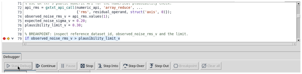
GUI debugger paused before checking the noise RMS — GNU Octave pauses at the native debugger breakpoint on the residual RMS plausibility check.

Execution pauses before the conditional check. Open Stack and variables to inspect the local values:

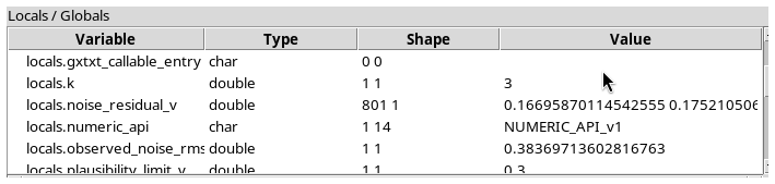
Debugger variable observed_noise_rms_v reads 0.383697 V — The debugger highlights an RMS of approximately 0.384 V, caused by calculating the residual using the wrong reference.

The calculated RMS is 0.383697 V, above the 0.30 V limit. Next, inspect reference_dataset_id:

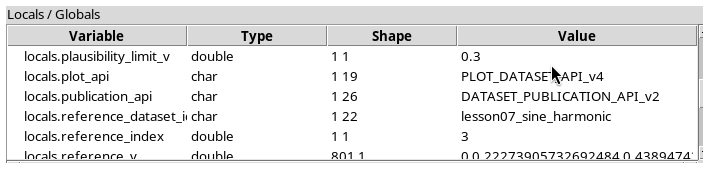
Debugger shows the harmonic signal chosen as reference Dataset — The reference_dataset_id variable identifies the harmonic signal selected incorrectly as the reference.

The variable contains lesson07_sine_harmonic instead of lesson07_sine_pure. The diagnosis is now supported by the data: we have subtracted a signal that includes a harmonic component unrelated to the noise.

Click Continue. The condition evaluates to true, and the script reaches the intentional exception:

GNU Octave script stopped at its expected error statement — After Continue, the deliberately incorrect script reaches the statement that raises the exception.

Noise RMS 0.38370 V exceeds 0.30 V; check reference Dataset lesson07_sine_harmonic.

The diagnostic message reports an RMS of 0.38370 V, above the 0.30 V limit.

A debugger can therefore be used to inspect scientific decisions—reference selection, units, alignment, and assumptions—not merely to fix syntax errors. Here, the failed execution is expected and useful: it prevents a wrongly interpreted residual from being published.

8. Correcting the Reference and Interpreting the Statistics

Import L09_02_Descriptive_Statistics_Correct.m and choose a new Script ID. The correction is to select the physically appropriate reference:

reference_dataset_id = 'lesson07_sine_pure'; % Correct physical reference.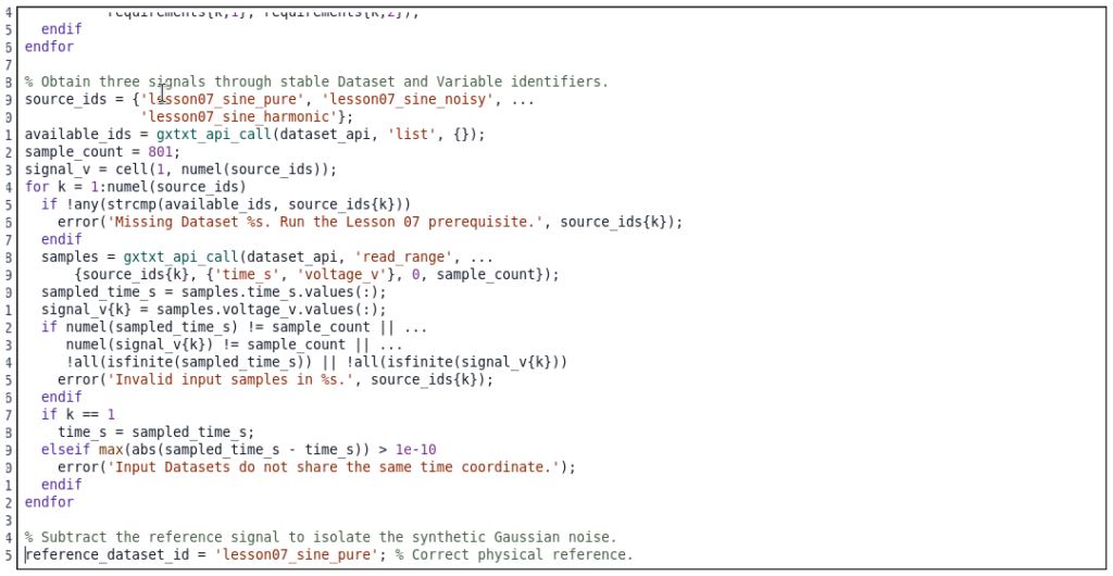

Corrected source selects lesson07_sine_pure as the reference — The corrected program subtracts the pure reference signal, isolating the synthetic noise.

Run the script using Run → Open Script Runner → Run Job. The Job Manager confirms completion, and the program reports the following values:

The corrected GNU Octave script finishes successfully in the framework Job Manager.

Statistic	Value	Unit / interpretation
Number of observations	801	samples
Mean residual	−0.005805	V
Median residual	−0.003924	V
Sample standard deviation	0.206560	V
Population standard deviation	0.206431	V
Sample variance	0.04266717	V²
Residual RMS	0.206513	V
Standard error of the mean	0.007298	V, assuming independent observations

The generator’s nominal standard deviation was 0.20 V, but a finite sequence need not exactly reproduce the theoretical distribution parameter. Since the mean is close to zero, RMS and population standard deviation are almost equal. Under the assumptions already discussed, SEM describes the statistical precision of the mean; it is not a statement about instrumental accuracy or measurement uncertainty.

The program also compares Numeric API reductions with native GNU Octave expressions. For these arrays, the results agree within the specified numerical tolerances. This comparison checks the numerical calculations, but does not replace reasoning about what the data mean.

9. Running Mean, Sorting, and Empirical Cumulative Distribution

9.1 The `cumsum()` Function and the Running Mean

The cumsum(v) function returns a vector of cumulative sums: each position contains the sum of observations up to that point. Dividing each cumulative sum by the number of observations collected so far gives the running mean.

values_v = [2; 4; 6; 8];
running_sum = cumsum(values_v);               % [2; 6; 12; 20]
running_mean = running_sum ./ (1:numel(values_v))';  % [2; 3; 4; 5]

The ./ operator performs element-wise division. The transpose operator ' turns the divisor sequence into a column vector compatible with the output of cumsum. In our script:

running_mean_v = cumsum(noise_residual_v) ./ (1:sample_count)';

The running mean helps us examine how an estimate evolves, but it does not by itself establish that a sequence is independent, stationary, or sufficiently long. A visually flattening curve is not proof of statistical convergence.

9.2 The `sort()` Function and the ECDF

The sort function arranges samples from smallest to largest. Associating the observation at sorted position k with the fraction k/N lets us construct an empirical cumulative distribution function (ECDF). Its mathematical definition is:

F_N(x)=\frac{1}{N}\sum_{i=1}^{N}\mathbf{1}_{\{r_i\le x\}}.

The indicator \(\mathbf{1}_{\{r_i\le x\}}\) equals 1 when the sample is no greater than x, and 0 otherwise. Thus, F_N(x) measures the fraction of observations less than or equal to the threshold x. It does not require assuming a normal distribution in advance.

values_v = [3; -2; 1; 0];
ordered_v = sort(values_v);       % [-2; 0; 1; 3]
n = numel(ordered_v);            % 4
cdf_fraction = (1:n)' / n;        % [0.25; 0.50; 0.75; 1.00]

The full ECDF is theoretically a step function, with jumps at the observed values. The script displays the ordered points as a curve: for continuous data without ties, the trend is easy to read; when observations repeat, care is needed to interpret the vertical jumps in the cumulative distribution. The S-shaped profile in our example is compatible with the Gaussian-noise model, but it is not a formal normality test.

9.3 Publishing New Datasets and Using Plot Dataset

The program publishes three derived Datasets through DATASET_PUBLICATION_API_v2/publish_series_batch, retaining their variable identities, units, and relationships to the original data. The results are then accessible to other GX-TXT tools.

Published Dataset	X variable	Y variable
`lesson09_noise_residual`	`time_s`	`residual_v`
`lesson09_running_mean`	`time_s`	`running_mean_v`
`lesson09_noise_ecdf`	`residual_v`	`fraction`

In the GX-TXT Plots tab, the first variant displays the noise residual and its running mean on the same time axis:

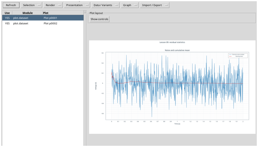
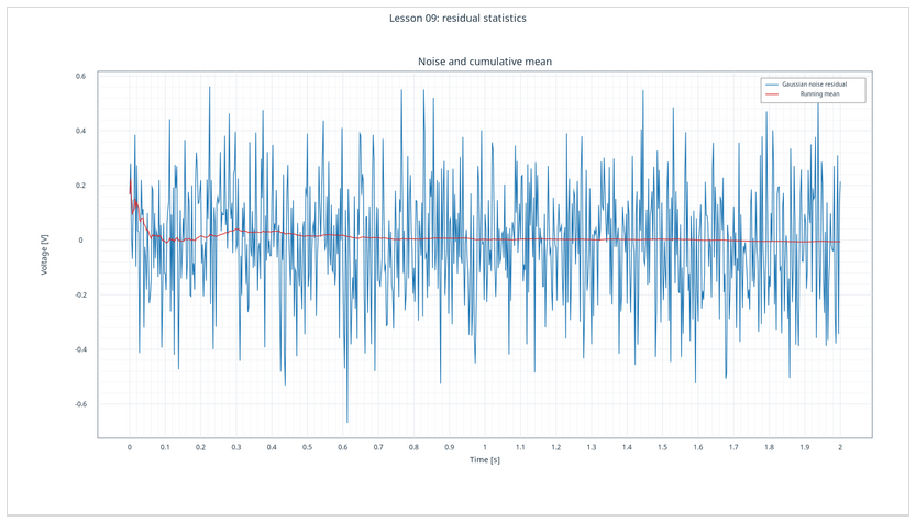
Native GX-TXT time plot of noise residual and running average — The noise residual and running mean are displayed through GX-TXT Plot Dataset API v4.

Focused screenshot of the synthetic noise voltage residual and running mean — A close-up of the native GX-TXT noise-residual plot.

The fluctuations remain around zero, while the running mean approaches the small average value of the series. The second variant shows the empirical cumulative distribution of the noise as a function of voltage:

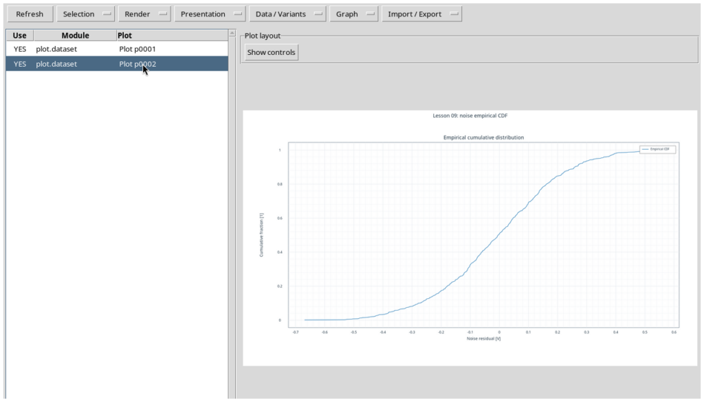
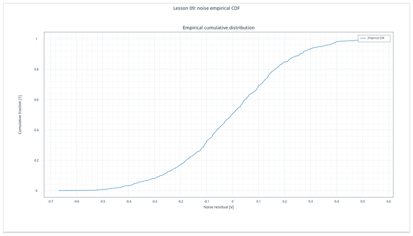
Native GX-TXT empirical cumulative distribution graph of voltage noise — The second persistent plot variant shows the empirical cumulative distribution of the noise.

Focused native GX-TXT chart of cumulative probability versus noise voltage — A detailed view of the empirical cumulative distribution calculated from 801 samples.

The ECDF describes the observed samples. Assessing quantitative agreement with a theoretical distribution would require additional tools, such as a comparison with theoretical quantiles or an appropriate statistical test, which are beyond the scope of this lesson.

10. Reproducibility and Limitations of the Experiment

The procedure is reproducible because the signal model, sampling rate, number of samples, pseudorandom seed, and numerical operations are specified. The program detects the incorrect reference choice, calculates statistics with the corrected version, and makes the Datasets and plots available in the same Session.

An identical seed reproduces the same sequence only with a compatible generator and runtime. The descriptive statistics characterize this synthetic realization; they do not certify the performance of a physical instrument. Further topics include possible temporal correlation, systematic errors, confidence intervals, measurement uncertainty, and quantitative comparison with a probabilistic model.

11. Practice Exercises

Using the vector [2;4;6;8], manually verify the sum of squared deviations and calculate both variances in Octave. Explain the role of N − 1.
Change the generator’s standard deviation from 0.20 V to 0.10 V, repeat the procedure in a new Session, and compare the new RMS and standard-deviation results.
Demonstrate numerically that rms(v)^2 = var(v,1) + mean(v)^2, computing RMS with the Octave expression sqrt(mean(v.^2)).
Compare std(v,0) with std(v,1) and explain why their difference depends on the number of samples.
Manually construct the running mean for [2;4;6;8] and compare it with cumsum(v)./(1:numel(v))'.
Construct the ECDF points for [-2;0;1;3] and interpret F_N(0). Repeat with two equal observations and identify the resulting jump.
Repeat the signal generation with a different seed and distinguish changes in sample estimates from changes in theoretical distribution parameters.
Replace the correct reference Dataset with the harmonic Dataset. Which checks still pass, and which one reveals that the residual has been given the wrong physical meaning?

In Lesson 10, we will move from descriptive analysis to interpolation and fitting, introducing mathematical models to explain and predict relationships between experimental quantities.

12. Lesson Materials and Documentation

The three complete scripts are provided in the next section inside collapsible panels. The first generates the input Datasets; the second contains an intentional scientific error; and the third performs the correct calculations, publishes the results, and creates the two GX-TXT plots. Comments within the scripts remain in English, as throughout the course.

Public API references: Octave Script Bridge v1; Canonical Dataset v2; Numeric API v1; Dataset Publication v2; Plot Dataset v4.

13. Complete GNU Octave Scripts

Select each panel’s title to show or hide the complete source code. Import the scripts into GX-TXT’s Octave Script Workspace in the order shown; run the buggy script in the debugger and the corrected version through the Script Runner.

Script 1 — Generate the Three Synthetic Signals (Prerequisite)

File: L09_00_Prerequisite_L07_Signals.m · GNU Octave · comments in English · GPL-3.0-or-later.

% Lesson 07.02 - Publish three synthetic signals in one atomic batch.
% SPDX-License-Identifier: GPL-3.0-or-later
%
% GX-TXT reference: DEV112-P005
% GitHub branch: maintenance/dev112
% Reference commit: 125afdb62110a92199f59a066199bb7f2dc7ed68
%
% Run from the GX-TXT GNU Octave Script Workspace.
% Each Dataset has its own stable identity, schema, and metadata.
% The entire batch is create-only and atomic: any failed publication
% leaves none of the three new Datasets registered.
%
% Use a new Session or change all three IDs before repeating this script.

% The GX-TXT runner already isolates this script's variable workspace.
% Do not use clear here: it would erase the runner's local arguments.

% Step 1: Generate three related 5 Hz signals with a common time axis.
sample_rate_hz = 400;
duration_s = 2;
frequency_hz = 5;
amplitude_v = 1.5;
noise_standard_deviation_v = 0.2;
third_harmonic_amplitude_v = 0.45;

time_s = (0:(sample_rate_hz * duration_s))' / sample_rate_hz;
sample_count = numel(time_s);

rng(707, 'twister');
pure_v = amplitude_v * sin(2 * pi * frequency_hz * time_s);
noisy_v = pure_v + noise_standard_deviation_v * randn(sample_count, 1);
harmonic_v = pure_v + ...
    third_harmonic_amplitude_v * sin(2 * pi * (3 * frequency_hz) * time_s);

signal_values = {pure_v, noisy_v, harmonic_v};
dataset_ids = {'lesson07_sine_pure', 'lesson07_sine_noisy', ...
               'lesson07_sine_harmonic'};
model_labels = {'pure sinusoid', 'sinusoid with Gaussian noise', ...
                'sinusoid with third harmonic'};

for k = 1:numel(signal_values)
  assert(iscolumn(signal_values{k}));
  assert(numel(signal_values{k}) == sample_count);
  assert(all(isfinite(signal_values{k})));
endfor

% Step 2: Verify the public batch writer and public Dataset reader.
publication_api = 'DATASET_PUBLICATION_API_v2';
dataset_api = 'CANONICAL_DATASET_API_v2';
gxtxt_api_require({publication_api, dataset_api});

if !gxtxt_api_has_operation(publication_api, 'publish_series_batch')
  error('The public atomic batch publication operation is unavailable.');
endif

for operation = {'list', 'read_range'}
  if !gxtxt_api_has_operation(dataset_api, operation{1})
    error('Missing Dataset read operation: %s', operation{1});
  endif
endfor

existing_ids = gxtxt_api_call(dataset_api, 'list', {});
for k = 1:numel(dataset_ids)
  if any(strcmp(existing_ids, dataset_ids{k}))
    error('Dataset "%s" already exists. No batch was submitted.', dataset_ids{k});
  endif
endfor

% Step 3: Build the shared Variable Schema v3 declarations.
time_variable = struct( ...
    'variable_id', 'time_s', ...
    'name', 'time_s', ...
    'display_label', 'Elapsed time', ...
    'unit', 's', ...
    'dtype', 'float64', ...
    'value_kind', 'number', ...
    'semantic_role', 'time', ...
    'semantic_source', 'generator');

voltage_variable = struct( ...
    'variable_id', 'voltage_v', ...
    'name', 'voltage_v', ...
    'display_label', 'Simulated voltage', ...
    'unit', 'V', ...
    'dtype', 'float64', ...
    'value_kind', 'number', ...
    'semantic_role', 'voltage', ...
    'semantic_source', 'generator');

% Step 4: Give each output its own scientific metadata and samples.
series_requests = cell(1, numel(dataset_ids));

for k = 1:numel(dataset_ids)
  metadata = struct();
  metadata.('simulation.model') = model_labels{k};
  metadata.('simulation.frequency_hz') = frequency_hz;
  metadata.('simulation.sample_rate_hz') = sample_rate_hz;
  metadata.('simulation.random_seed') = 707;
  metadata.('simulation.noise_std_v') = ...
      (k == 2) * noise_standard_deviation_v;
  metadata.('simulation.third_harmonic_v') = ...
      (k == 3) * third_harmonic_amplitude_v;

  series_requests{k} = struct( ...
      'dataset_id', dataset_ids{k}, ...
      'contract', 'table.generic', ...
      'storage', 'auto', ...
      'x_values', time_s, ...
      'y_values', signal_values{k}, ...
      'x_variable', time_variable, ...
      'y_variable', voltage_variable, ...
      'producer_version', '1.0.0', ...
      'source', 'GNU Octave synthetic signal generator', ...
      'provenance', 'Reproducible Lesson 07 synthetic signal', ...
      'notes', model_labels{k}, ...
      'structured_metadata', metadata);
endfor

% Step 5: Request an atomic publication of all three separate Datasets.
batch_request = struct();
batch_request.series = series_requests;

receipt = gxtxt_api_call(publication_api, 'publish_series_batch', ...
                         {batch_request});

if !receipt.atomic || receipt.output_count != numel(dataset_ids)
  error('The batch publication receipt did not confirm three atomic outputs.');
endif

% Step 6: Verify each published Variable using the public read API.
published_ids = gxtxt_api_call(dataset_api, 'list', {});
for k = 1:numel(dataset_ids)
  assert(any(strcmp(published_ids, dataset_ids{k})));

  samples = gxtxt_api_call(dataset_api, 'read_range', ...
      {dataset_ids{k}, {'time_s', 'voltage_v'}, 0, sample_count});

  read_time_s = samples.time_s.values(:);
  read_voltage_v = samples.voltage_v.values(:);

  assert(numel(read_time_s) == sample_count);
  assert(numel(read_voltage_v) == sample_count);

  time_error = max(abs(read_time_s - time_s));
  voltage_error = max(abs(read_voltage_v - signal_values{k}));

  if time_error > 1e-9 || voltage_error > 1e-9
    error('Read-back verification failed for Dataset "%s".', dataset_ids{k});
  endif

  fprintf('Verified Dataset: %-27s %4d samples, max error %.3g V\n', ...
          dataset_ids{k}, sample_count, voltage_error);
endfor

fprintf('Atomic publication succeeded for %d Datasets.\n', ...
        receipt.output_count);

Script 2 — Deliberately Incorrect Reference (Debugging Exercise)

File: L09_01_Debug_Wrong_Reference.m · GNU Octave · comments in English · GPL-3.0-or-later.

% Lesson 09 - Descriptive statistics for experimental signal residuals
% Course: GNU Octave with GX-TXT | GX-TXT DEV112-P005
% GitHub reference: maintenance/dev112
% Source commit: 125afdb62110a92199f59a066199bb7f2dc7ed68
% SPDX-License-Identifier: GPL-3.0-or-later
%
% Run as a GX-TXT managed GNU Octave Session script.
% Prerequisite: the three Lesson 07 signals have been published.
% The Script Bridge is managed by GX-TXT; do not start it manually.
% All Dataset and plot operations use public framework APIs.
% Use a new Session: derived Dataset IDs are intentionally create-only.

dataset_api = 'CANONICAL_DATASET_API_v2';
numeric_api = 'NUMERIC_API_v1';
publication_api = 'DATASET_PUBLICATION_API_v2';
plot_api = 'PLOT_DATASET_API_v4';
gxtxt_api_require({dataset_api, numeric_api, publication_api, plot_api});

requirements = {
  dataset_api, 'list';
  dataset_api, 'read_range';
  numeric_api, 'array_reduce';
  numeric_api, 'statistics';
  publication_api, 'publish_series_batch';
  plot_api, 'new_spec';
  plot_api, 'validate_spec';
  plot_api, 'upsert_plot';
  plot_api, 'render';
  plot_api, 'artifacts'
};
for k = 1:rows(requirements)
  if !gxtxt_api_has_operation(requirements{k,1}, requirements{k,2})
    error('Missing public operation %s/%s.', ...
          requirements{k,1}, requirements{k,2});
  endif
endfor

% Obtain three signals through stable Dataset and Variable identifiers.
source_ids = {'lesson07_sine_pure', 'lesson07_sine_noisy', ...
              'lesson07_sine_harmonic'};
available_ids = gxtxt_api_call(dataset_api, 'list', {});
sample_count = 801;
signal_v = cell(1, numel(source_ids));
for k = 1:numel(source_ids)
  if !any(strcmp(available_ids, source_ids{k}))
    error('Missing Dataset %s. Run the Lesson 07 prerequisite.', source_ids{k});
  endif
  samples = gxtxt_api_call(dataset_api, 'read_range', ...
      {source_ids{k}, {'time_s', 'voltage_v'}, 0, sample_count});
  sampled_time_s = samples.time_s.values(:);
  signal_v{k} = samples.voltage_v.values(:);
  if numel(sampled_time_s) != sample_count || ...
     numel(signal_v{k}) != sample_count || ...
     !all(isfinite(sampled_time_s)) || !all(isfinite(signal_v{k}))
    error('Invalid input samples in %s.', source_ids{k});
  endif
  if k == 1
    time_s = sampled_time_s;
  elseif max(abs(sampled_time_s - time_s)) > 1e-10
    error('Input Datasets do not share the same time coordinate.');
  endif
endfor

% Subtract the reference signal to isolate the synthetic Gaussian noise.
reference_dataset_id = 'lesson07_sine_harmonic'; % INTENTIONAL BUG: use the pure signal.
reference_index = find(strcmp(source_ids, reference_dataset_id));
reference_v = signal_v{reference_index};
noise_residual_v = signal_v{2} - reference_v;
residual_operand = struct('kind', 'vector', 'value', noise_residual_v);

% Use GX-TXT's public Numeric API for the numerical plausibility check.
api_rms = gxtxt_api_call(numeric_api, 'array_reduce', ...
                         {'rms', residual_operand, struct('axis', 0)});
observed_noise_rms_v = api_rms.values(1);
expected_noise_sigma_v = 0.20;
plausibility_limit_v = 0.30;

% BREAKPOINT: inspect reference_dataset_id, observed_noise_rms_v and the limit.
if observed_noise_rms_v > plausibility_limit_v
  error('Noise RMS %.5f V exceeds %.2f V; check reference Dataset %s.', ...
        observed_noise_rms_v, plausibility_limit_v, reference_dataset_id);
endif

% Compare native Octave statistics with the public numerical operations.
api_mean = gxtxt_api_call(numeric_api, 'array_reduce', ...
                          {'mean', residual_operand, struct('axis', 0)});
api_sample_std = gxtxt_api_call(numeric_api, 'array_reduce', ...
                                {'std_sample', residual_operand, struct('axis', 0)});
api_statistics = gxtxt_api_call(numeric_api, 'statistics', ...
                                {noise_residual_v, struct()});
mean_v = mean(noise_residual_v);
median_v = median(noise_residual_v);
population_std_v = std(noise_residual_v, 1);
sample_std_v = std(noise_residual_v, 0);
variance_sample_v2 = var(noise_residual_v, 0);
rms_native_v = sqrt(mean(noise_residual_v .^ 2));
standard_error_v = sample_std_v / sqrt(sample_count);
assert(abs(api_mean.values(1) - mean_v) < 1e-10);
assert(abs(api_sample_std.values(1) - sample_std_v) < 1e-9);
assert(abs(observed_noise_rms_v - rms_native_v) < 1e-10);

% The empirical CDF is monotone and uses original residual values.
sorted_noise_v = sort(noise_residual_v);
cumulative_fraction = (1:sample_count)' / sample_count;
running_mean_v = cumsum(noise_residual_v) ./ (1:sample_count)';

fprintf('Descriptive statistics: %d synthetic noise residuals\n', sample_count);
fprintf('Mean = %.6f V; median = %.6f V\n', mean_v, median_v);
fprintf('Sample SD = %.6f V; population SD = %.6f V\n', ...
        sample_std_v, population_std_v);
fprintf('Sample variance = %.8f V^2; RMS = %.6f V\n', ...
        variance_sample_v2, observed_noise_rms_v);
fprintf('SEM = %.6f V (assumes independent observations)\n', ...
        standard_error_v);
disp('GX-TXT Numeric API statistics receipt:');
disp(api_statistics);

% Publish three independent derived scientific Datasets atomically.
derived_ids = {'lesson09_noise_residual', 'lesson09_running_mean', ...
               'lesson09_noise_ecdf'};
existing_ids = gxtxt_api_call(dataset_api, 'list', {});
for k = 1:numel(derived_ids)
  if any(strcmp(existing_ids, derived_ids{k}))
    error('Derived Dataset %s already exists: use a fresh Session.', derived_ids{k});
  endif
endfor

time_variable = struct('variable_id', 'time_s', 'name', 'time_s', ...
    'display_label', 'Elapsed time', 'unit', 's', 'dtype', 'float64', ...
    'value_kind', 'number', 'semantic_role', 'time', ...
    'semantic_source', 'plugin');
residual_variable = struct('variable_id', 'residual_v', ...
    'name', 'residual_v', 'display_label', 'Noise residual', ...
    'unit', 'V', 'dtype', 'float64', 'value_kind', 'number', ...
    'semantic_role', 'voltage', 'semantic_source', 'plugin');
mean_variable = struct('variable_id', 'running_mean_v', ...
    'name', 'running_mean_v', 'display_label', 'Running mean', ...
    'unit', 'V', 'dtype', 'float64', 'value_kind', 'number', ...
    'semantic_role', 'voltage', 'semantic_source', 'plugin');
fraction_variable = struct('variable_id', 'fraction', ...
    'name', 'fraction', 'display_label', 'Empirical cumulative fraction', ...
    'unit', '1', 'dtype', 'float64', 'value_kind', 'number', ...
    'semantic_role', 'fraction', 'semantic_source', 'plugin');

x_values = {time_s, time_s, sorted_noise_v};
y_values = {noise_residual_v, running_mean_v, cumulative_fraction};
x_variables = {time_variable, time_variable, residual_variable};
y_variables = {residual_variable, mean_variable, fraction_variable};
descriptions = {'Noise residual vs time', ...
                'Running mean of the noise residual', ...
                'Empirical cumulative distribution of noise residuals'};
series_requests = cell(1, numel(derived_ids));
for k = 1:numel(derived_ids)
  metadata = struct();
  metadata.('analysis.kind') = descriptions{k};
  metadata.('analysis.reference_dataset') = reference_dataset_id;
  metadata.('analysis.input_samples') = sample_count;
  metadata.('analysis.expected_noise_sigma_v') = expected_noise_sigma_v;
  metadata.('analysis.sample_std_v') = sample_std_v;
  series_requests{k} = struct( ...
      'dataset_id', derived_ids{k}, 'contract', 'table.generic', ...
      'storage', 'auto', 'x_values', x_values{k}, ...
      'y_values', y_values{k}, ...
      'x_variable', x_variables{k}, 'y_variable', y_variables{k}, ...
      'producer_version', '1.0.0', ...
      'source', 'GX-TXT Octave Lesson 09', ...
      'provenance', 'Derived from Lesson 07 canonical signals', ...
      'source_dataset_ids', {source_ids}, ...
      'notes', descriptions{k}, 'structured_metadata', metadata);
endfor
batch = struct('series', {series_requests});
receipt = gxtxt_api_call(publication_api, 'publish_series_batch', {batch});
if !receipt.atomic || receipt.output_count != numel(derived_ids)
  error('Atomic publication did not confirm three derived Datasets.');
endif

% Read derived values back from the public canonical Dataset API.
published = gxtxt_api_call(dataset_api, 'list', {});
for k = 1:numel(derived_ids)
  if !any(strcmp(published, derived_ids{k}))
    error('Published Dataset %s is absent.', derived_ids{k});
  endif
  saved = gxtxt_api_call(dataset_api, 'read_range', ...
      {derived_ids{k}, ...
       {x_variables{k}.variable_id, y_variables{k}.variable_id}, ...
       0, sample_count});
  recovered = saved.(y_variables{k}.variable_id).values(:);
  if max(abs(recovered - y_values{k})) > 1e-9
    error('Read-back mismatch for %s.', derived_ids{k});
  endif
endfor

% Plot 1: noise residual and its running mean on a single GX-TXT plot.
trend = gxtxt_api_call(plot_api, 'new_spec', ...
                       {'plot.dataset.xy', 'Lesson 09: residual statistics'});
panel = trend.panels{1};
panel.id = 'noise_overview';
panel.title = 'Noise and cumulative mean';
panel.axes = struct('x', struct('label', 'Time [s]', 'scale', 'linear'), ...
    'y_left', struct('label', 'Voltage [V]', 'scale', 'linear'));
panel.series = {
  struct('id', 'noise', 'label', 'Gaussian noise residual', ...
         'dataset_id', derived_ids{1}, 'x_variable_id', 'time_s', ...
         'y_variable_id', 'residual_v', 'axis', 'left', 'kind', 'line'),
  struct('id', 'running_mean', 'label', 'Running mean', ...
         'dataset_id', derived_ids{2}, 'x_variable_id', 'time_s', ...
         'y_variable_id', 'running_mean_v', 'axis', 'left', 'kind', 'line')
};
trend.panels = {panel};
if !gxtxt_api_call(plot_api, 'validate_spec', {trend})
  error('Residual PlotSpec failed public validation.');
endif
trend_ref = gxtxt_api_call(plot_api, 'upsert_plot', ...
                           {'lesson09_noise_overview', trend});
gxtxt_api_call(plot_api, 'render', {trend_ref});
trend_artifacts = gxtxt_api_call(plot_api, 'artifacts', {trend_ref});

% Plot 2: empirical cumulative distribution of the observed noise.
distribution = gxtxt_api_call(plot_api, 'new_spec', ...
                       {'plot.dataset.xy', 'Lesson 09: noise empirical CDF'});
cdf_panel = distribution.panels{1};
cdf_panel.id = 'noise_cdf';
cdf_panel.title = 'Empirical cumulative distribution';
cdf_panel.axes = struct( ...
    'x', struct('label', 'Noise residual [V]', 'scale', 'linear'), ...
    'y_left', struct('label', 'Cumulative fraction [1]', 'scale', 'linear'));
cdf_panel.series = {struct( ...
    'id', 'ecdf', 'label', 'Empirical CDF', ...
    'dataset_id', derived_ids{3}, ...
    'x_variable_id', 'residual_v', 'y_variable_id', 'fraction', ...
    'axis', 'left', 'kind', 'line')};
distribution.panels = {cdf_panel};
if !gxtxt_api_call(plot_api, 'validate_spec', {distribution})
  error('Empirical-CDF PlotSpec failed public validation.');
endif
cdf_ref = gxtxt_api_call(plot_api, 'upsert_plot', ...
                         {'lesson09_noise_ecdf', distribution});
gxtxt_api_call(plot_api, 'render', {cdf_ref});
cdf_artifacts = gxtxt_api_call(plot_api, 'artifacts', {cdf_ref});

fprintf('PASS: 3 canonical derived Datasets and 2 persistent GX-TXT plots.\n');
disp(trend_artifacts);
disp(cdf_artifacts);

Script 3 — Descriptive Statistics, Datasets and Plots (Correct Version)

File: L09_02_Descriptive_Statistics_Correct.m · GNU Octave · comments in English · GPL-3.0-or-later.

% Lesson 09 - Descriptive statistics for experimental signal residuals
% Course: GNU Octave with GX-TXT | GX-TXT DEV112-P005
% GitHub reference: maintenance/dev112
% Source commit: 125afdb62110a92199f59a066199bb7f2dc7ed68
% SPDX-License-Identifier: GPL-3.0-or-later
%
% Run as a GX-TXT managed GNU Octave Session script.
% Prerequisite: the three Lesson 07 signals have been published.
% The Script Bridge is managed by GX-TXT; do not start it manually.
% All Dataset and plot operations use public framework APIs.
% Use a new Session: derived Dataset IDs are intentionally create-only.

dataset_api = 'CANONICAL_DATASET_API_v2';
numeric_api = 'NUMERIC_API_v1';
publication_api = 'DATASET_PUBLICATION_API_v2';
plot_api = 'PLOT_DATASET_API_v4';
gxtxt_api_require({dataset_api, numeric_api, publication_api, plot_api});

requirements = {
  dataset_api, 'list';
  dataset_api, 'read_range';
  numeric_api, 'array_reduce';
  numeric_api, 'statistics';
  publication_api, 'publish_series_batch';
  plot_api, 'new_spec';
  plot_api, 'validate_spec';
  plot_api, 'upsert_plot';
  plot_api, 'render';
  plot_api, 'artifacts'
};
for k = 1:rows(requirements)
  if !gxtxt_api_has_operation(requirements{k,1}, requirements{k,2})
    error('Missing public operation %s/%s.', ...
          requirements{k,1}, requirements{k,2});
  endif
endfor

% Obtain three signals through stable Dataset and Variable identifiers.
source_ids = {'lesson07_sine_pure', 'lesson07_sine_noisy', ...
              'lesson07_sine_harmonic'};
available_ids = gxtxt_api_call(dataset_api, 'list', {});
sample_count = 801;
signal_v = cell(1, numel(source_ids));
for k = 1:numel(source_ids)
  if !any(strcmp(available_ids, source_ids{k}))
    error('Missing Dataset %s. Run the Lesson 07 prerequisite.', source_ids{k});
  endif
  samples = gxtxt_api_call(dataset_api, 'read_range', ...
      {source_ids{k}, {'time_s', 'voltage_v'}, 0, sample_count});
  sampled_time_s = samples.time_s.values(:);
  signal_v{k} = samples.voltage_v.values(:);
  if numel(sampled_time_s) != sample_count || ...
     numel(signal_v{k}) != sample_count || ...
     !all(isfinite(sampled_time_s)) || !all(isfinite(signal_v{k}))
    error('Invalid input samples in %s.', source_ids{k});
  endif
  if k == 1
    time_s = sampled_time_s;
  elseif max(abs(sampled_time_s - time_s)) > 1e-10
    error('Input Datasets do not share the same time coordinate.');
  endif
endfor

% Subtract the reference signal to isolate the synthetic Gaussian noise.
reference_dataset_id = 'lesson07_sine_pure'; % Correct physical reference.
reference_index = find(strcmp(source_ids, reference_dataset_id));
reference_v = signal_v{reference_index};
noise_residual_v = signal_v{2} - reference_v;
residual_operand = struct('kind', 'vector', 'value', noise_residual_v);

% Use GX-TXT's public Numeric API for the numerical plausibility check.
api_rms = gxtxt_api_call(numeric_api, 'array_reduce', ...
                         {'rms', residual_operand, struct('axis', 0)});
observed_noise_rms_v = api_rms.values(1);
expected_noise_sigma_v = 0.20;
plausibility_limit_v = 0.30;

% BREAKPOINT: inspect reference_dataset_id, observed_noise_rms_v and the limit.
if observed_noise_rms_v > plausibility_limit_v
  error('Noise RMS %.5f V exceeds %.2f V; check reference Dataset %s.', ...
        observed_noise_rms_v, plausibility_limit_v, reference_dataset_id);
endif

% Compare native Octave statistics with the public numerical operations.
api_mean = gxtxt_api_call(numeric_api, 'array_reduce', ...
                          {'mean', residual_operand, struct('axis', 0)});
api_sample_std = gxtxt_api_call(numeric_api, 'array_reduce', ...
                                {'std_sample', residual_operand, struct('axis', 0)});
api_statistics = gxtxt_api_call(numeric_api, 'statistics', ...
                                {noise_residual_v, struct()});
mean_v = mean(noise_residual_v);
median_v = median(noise_residual_v);
population_std_v = std(noise_residual_v, 1);
sample_std_v = std(noise_residual_v, 0);
variance_sample_v2 = var(noise_residual_v, 0);
rms_native_v = sqrt(mean(noise_residual_v .^ 2));
standard_error_v = sample_std_v / sqrt(sample_count);
assert(abs(api_mean.values(1) - mean_v) < 1e-10);
assert(abs(api_sample_std.values(1) - sample_std_v) < 1e-9);
assert(abs(observed_noise_rms_v - rms_native_v) < 1e-10);

% The empirical CDF is monotone and uses original residual values.
sorted_noise_v = sort(noise_residual_v);
cumulative_fraction = (1:sample_count)' / sample_count;
running_mean_v = cumsum(noise_residual_v) ./ (1:sample_count)';

fprintf('Descriptive statistics: %d synthetic noise residuals\n', sample_count);
fprintf('Mean = %.6f V; median = %.6f V\n', mean_v, median_v);
fprintf('Sample SD = %.6f V; population SD = %.6f V\n', ...
        sample_std_v, population_std_v);
fprintf('Sample variance = %.8f V^2; RMS = %.6f V\n', ...
        variance_sample_v2, observed_noise_rms_v);
fprintf('SEM = %.6f V (assumes independent observations)\n', ...
        standard_error_v);
disp('GX-TXT Numeric API statistics receipt:');
disp(api_statistics);

% Publish three independent derived scientific Datasets atomically.
derived_ids = {'lesson09_noise_residual', 'lesson09_running_mean', ...
               'lesson09_noise_ecdf'};
existing_ids = gxtxt_api_call(dataset_api, 'list', {});
for k = 1:numel(derived_ids)
  if any(strcmp(existing_ids, derived_ids{k}))
    error('Derived Dataset %s already exists: use a fresh Session.', derived_ids{k});
  endif
endfor

time_variable = struct('variable_id', 'time_s', 'name', 'time_s', ...
    'display_label', 'Elapsed time', 'unit', 's', 'dtype', 'float64', ...
    'value_kind', 'number', 'semantic_role', 'time', ...
    'semantic_source', 'plugin');
residual_variable = struct('variable_id', 'residual_v', ...
    'name', 'residual_v', 'display_label', 'Noise residual', ...
    'unit', 'V', 'dtype', 'float64', 'value_kind', 'number', ...
    'semantic_role', 'voltage', 'semantic_source', 'plugin');
mean_variable = struct('variable_id', 'running_mean_v', ...
    'name', 'running_mean_v', 'display_label', 'Running mean', ...
    'unit', 'V', 'dtype', 'float64', 'value_kind', 'number', ...
    'semantic_role', 'voltage', 'semantic_source', 'plugin');
fraction_variable = struct('variable_id', 'fraction', ...
    'name', 'fraction', 'display_label', 'Empirical cumulative fraction', ...
    'unit', '1', 'dtype', 'float64', 'value_kind', 'number', ...
    'semantic_role', 'fraction', 'semantic_source', 'plugin');

x_values = {time_s, time_s, sorted_noise_v};
y_values = {noise_residual_v, running_mean_v, cumulative_fraction};
x_variables = {time_variable, time_variable, residual_variable};
y_variables = {residual_variable, mean_variable, fraction_variable};
descriptions = {'Noise residual vs time', ...
                'Running mean of the noise residual', ...
                'Empirical cumulative distribution of noise residuals'};
series_requests = cell(1, numel(derived_ids));
for k = 1:numel(derived_ids)
  metadata = struct();
  metadata.('analysis.kind') = descriptions{k};
  metadata.('analysis.reference_dataset') = reference_dataset_id;
  metadata.('analysis.input_samples') = sample_count;
  metadata.('analysis.expected_noise_sigma_v') = expected_noise_sigma_v;
  metadata.('analysis.sample_std_v') = sample_std_v;
  series_requests{k} = struct( ...
      'dataset_id', derived_ids{k}, 'contract', 'table.generic', ...
      'storage', 'auto', 'x_values', x_values{k}, ...
      'y_values', y_values{k}, ...
      'x_variable', x_variables{k}, 'y_variable', y_variables{k}, ...
      'producer_version', '1.0.0', ...
      'source', 'GX-TXT Octave Lesson 09', ...
      'provenance', 'Derived from Lesson 07 canonical signals', ...
      'source_dataset_ids', {source_ids}, ...
      'notes', descriptions{k}, 'structured_metadata', metadata);
endfor
batch = struct('series', {series_requests});
receipt = gxtxt_api_call(publication_api, 'publish_series_batch', {batch});
if !receipt.atomic || receipt.output_count != numel(derived_ids)
  error('Atomic publication did not confirm three derived Datasets.');
endif

% Read derived values back from the public canonical Dataset API.
published = gxtxt_api_call(dataset_api, 'list', {});
for k = 1:numel(derived_ids)
  if !any(strcmp(published, derived_ids{k}))
    error('Published Dataset %s is absent.', derived_ids{k});
  endif
  saved = gxtxt_api_call(dataset_api, 'read_range', ...
      {derived_ids{k}, ...
       {x_variables{k}.variable_id, y_variables{k}.variable_id}, ...
       0, sample_count});
  recovered = saved.(y_variables{k}.variable_id).values(:);
  if max(abs(recovered - y_values{k})) > 1e-9
    error('Read-back mismatch for %s.', derived_ids{k});
  endif
endfor

% Plot 1: noise residual and its running mean on a single GX-TXT plot.
trend = gxtxt_api_call(plot_api, 'new_spec', ...
                       {'plot.dataset.xy', 'Lesson 09: residual statistics'});
panel = trend.panels{1};
panel.id = 'noise_overview';
panel.title = 'Noise and cumulative mean';
panel.axes = struct('x', struct('label', 'Time [s]', 'scale', 'linear'), ...
    'y_left', struct('label', 'Voltage [V]', 'scale', 'linear'));
panel.series = {
  struct('id', 'noise', 'label', 'Gaussian noise residual', ...
         'dataset_id', derived_ids{1}, 'x_variable_id', 'time_s', ...
         'y_variable_id', 'residual_v', 'axis', 'left', 'kind', 'line'),
  struct('id', 'running_mean', 'label', 'Running mean', ...
         'dataset_id', derived_ids{2}, 'x_variable_id', 'time_s', ...
         'y_variable_id', 'running_mean_v', 'axis', 'left', 'kind', 'line')
};
trend.panels = {panel};
if !gxtxt_api_call(plot_api, 'validate_spec', {trend})
  error('Residual PlotSpec failed public validation.');
endif
trend_ref = gxtxt_api_call(plot_api, 'upsert_plot', ...
                           {'lesson09_noise_overview', trend});
gxtxt_api_call(plot_api, 'render', {trend_ref});
trend_artifacts = gxtxt_api_call(plot_api, 'artifacts', {trend_ref});

% Plot 2: empirical cumulative distribution of the observed noise.
distribution = gxtxt_api_call(plot_api, 'new_spec', ...
                       {'plot.dataset.xy', 'Lesson 09: noise empirical CDF'});
cdf_panel = distribution.panels{1};
cdf_panel.id = 'noise_cdf';
cdf_panel.title = 'Empirical cumulative distribution';
cdf_panel.axes = struct( ...
    'x', struct('label', 'Noise residual [V]', 'scale', 'linear'), ...
    'y_left', struct('label', 'Cumulative fraction [1]', 'scale', 'linear'));
cdf_panel.series = {struct( ...
    'id', 'ecdf', 'label', 'Empirical CDF', ...
    'dataset_id', derived_ids{3}, ...
    'x_variable_id', 'residual_v', 'y_variable_id', 'fraction', ...
    'axis', 'left', 'kind', 'line')};
distribution.panels = {cdf_panel};
if !gxtxt_api_call(plot_api, 'validate_spec', {distribution})
  error('Empirical-CDF PlotSpec failed public validation.');
endif
cdf_ref = gxtxt_api_call(plot_api, 'upsert_plot', ...
                         {'lesson09_noise_ecdf', distribution});
gxtxt_api_call(plot_api, 'render', {cdf_ref});
cdf_artifacts = gxtxt_api_call(plot_api, 'artifacts', {cdf_ref});

fprintf('PASS: 3 canonical derived Datasets and 2 persistent GX-TXT plots.\n');
disp(trend_artifacts);
disp(cdf_artifacts);

#data analysis #descriptive statistics #ECDF #GNU Octave #GX-TXT #Octave Debugger #public APIs #RMS #scientific programming #signal processing #standard deviation #variance

Lesson 09 — Descriptive Statistics and Debugging

1. Objectives and Links to Previous Lessons

2. The Experiment: Three Signals and a Physical Reference

3. Understanding Descriptive Statistics

3.1 Mean and Median: Two Measures of Central Tendency

3.2 Sample Variance, Population Variance, and Degrees of Freedom

3.3 Standard Deviation and RMS Are Not Synonyms

3.4 Standard Deviation and Standard Error of the Mean

3.5 Quartiles and the Interquartile Range

4. Implementing the Calculations with Octave and GX-TXT

4.1 Octave: Vector Operations

4.2 The Public NUMERIC_API_v1

4.3 Other APIs: Reading, Publishing, and Plotting

5. Preparing the Session and Generating the Input Datasets

6. An Intentional Scientific Logic Error

7. Finding the Error with the GNU Octave Debugger

8. Correcting the Reference and Interpreting the Statistics

9. Running Mean, Sorting, and Empirical Cumulative Distribution

9.1 The `cumsum()` Function and the Running Mean

9.2 The `sort()` Function and the ECDF

9.3 Publishing New Datasets and Using Plot Dataset

10. Reproducibility and Limitations of the Experiment

11. Practice Exercises

12. Lesson Materials and Documentation

13. Complete GNU Octave Scripts

Other steps of this project

Leave a Reply Cancel reply

Lesson 09 — Descriptive Statistics and Debugging

1. Objectives and Links to Previous Lessons

2. The Experiment: Three Signals and a Physical Reference

3. Understanding Descriptive Statistics

3.1 Mean and Median: Two Measures of Central Tendency

3.2 Sample Variance, Population Variance, and Degrees of Freedom

3.3 Standard Deviation and RMS Are Not Synonyms

3.4 Standard Deviation and Standard Error of the Mean

3.5 Quartiles and the Interquartile Range

4. Implementing the Calculations with Octave and GX-TXT

4.1 Octave: Vector Operations

4.2 The Public NUMERIC_API_v1

4.3 Other APIs: Reading, Publishing, and Plotting

5. Preparing the Session and Generating the Input Datasets

6. An Intentional Scientific Logic Error

7. Finding the Error with the GNU Octave Debugger

8. Correcting the Reference and Interpreting the Statistics

9. Running Mean, Sorting, and Empirical Cumulative Distribution

9.1 The cumsum() Function and the Running Mean

9.2 The sort() Function and the ECDF

9.3 Publishing New Datasets and Using Plot Dataset

10. Reproducibility and Limitations of the Experiment

11. Practice Exercises

12. Lesson Materials and Documentation

13. Complete GNU Octave Scripts

Other steps of this project

Leave a Reply Cancel reply

9.1 The `cumsum()` Function and the Running Mean

9.2 The `sort()` Function and the ECDF