

GX-TXT Debugger · Module 09 — Integrated practical cases
The GX-TXT debugger · 10-module course
If a chart or statistics appear plausible, the defect can be hidden in the previous steps. Here we follow the data path: sampling, missing values, residues, scale and publication. The six examples help to choose an intermediate control that makes clear the point where the result changes.
Download the Python and GNU Octave examples (ZIP). Extract all the archive folders and keep the multifile examples files together.
D49 — A time series with a skipped sample
A border error can exclude a sample from a temporal window. With small and identifiable data we can verify which positions enter the calculation before applying it to a wider range.
The same window in two languages
Consider five synthetic [10, 20, 30, 40, 50] samples. We want to select the second, third and fourth: the expected result is [20, 30, 40].
In slices.py, samples[1:4] uses zero indexes and exclusive final limit. Stop the press debugger: in the window test it has 3 length.
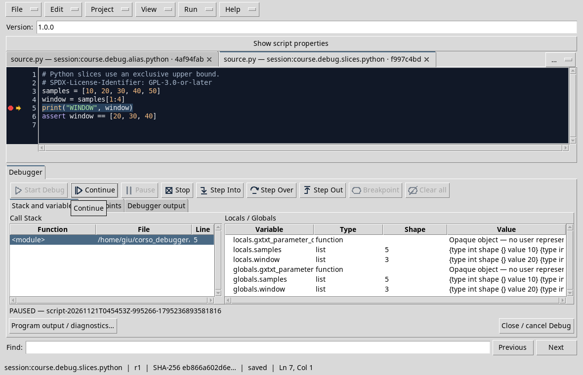
In indexing.m, the same window is samples(2:4): Octave starts from 1 and the range includes 4. The test stops before printing after reading the first sample and window.
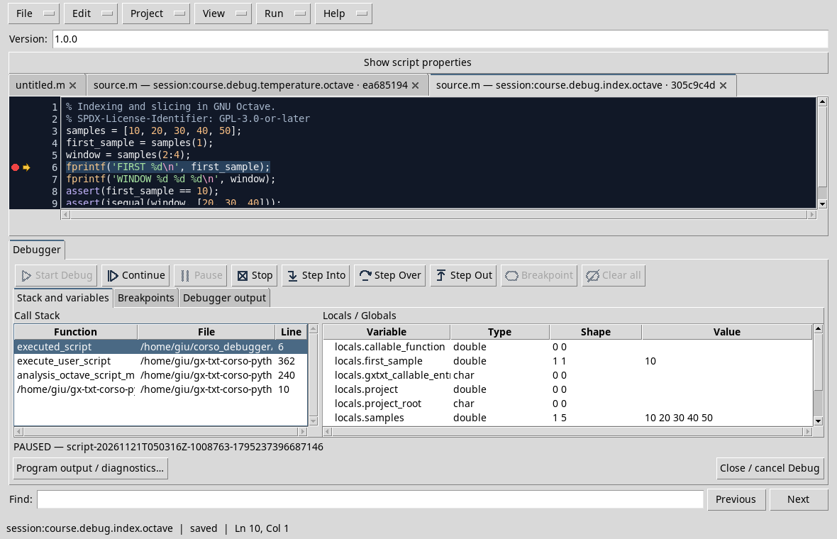
The correct form depends on the convention of language. If the requirement also included the fifth sample, it would have to change both intervals and the expected result; the debugger helps to verify the choice, but the requirement comes before the code.
Exercise
What expressions select 30 and 40 respectively in Python and Octave?
Worked solution
Python: samples[2:4]. Octave: samples(3:4). Both select the third and fourth sample.
Course index · Previous lesson
D50 — Statistics with missing values
An absent measure is not equivalent to a measure equal to zero. To make the distinction explicit, we use a mask of validity separated from the values.
Follow the filter
Import and record missing_mean.m in Octave Scripts. The samples = [2, 0, 4, 6] vector contains a placeholder in the second position; is_valid = [1, 0, 1, 1] indicates which observations are valid. The choice to exclude that position is declared by the mask, not deducted from the zero value.
Open View → Debugger, set a breakpoint on the press and start Start Debug. Check in Locals / Globals valid, valid_count and mean_valid: the expected results are [2, 4, 6], 3 and 4 respectively. The second position does not contribute to the average. Complete the Job with Continue.
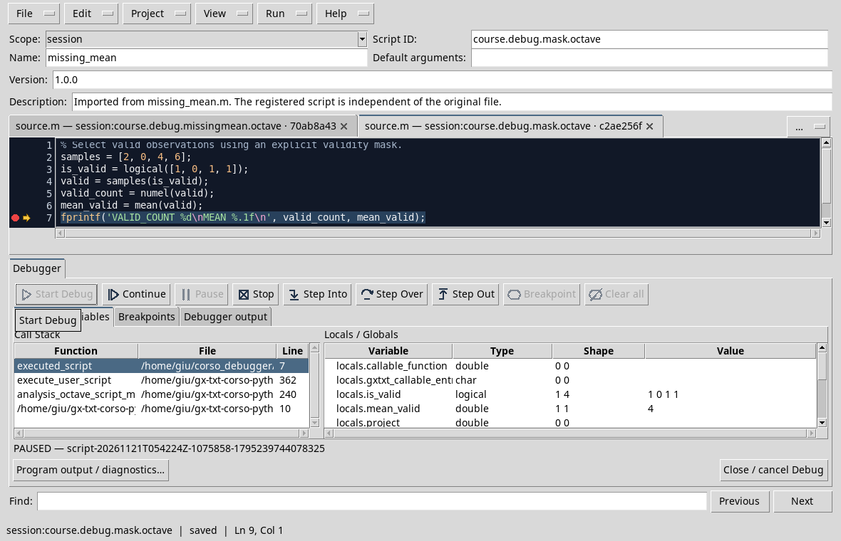
In the test the mask and the media are visible in Locals / Globals; scroll the panel to reach the other values. If your dataset uses another coding of missing values, build the mask according to its contract, without assuming that every zero is missing. Manage explicitly also the case where no element is valid.
Exercise
If all four positions were valid, what media would you get?
Worked solution
The average would be (2 + 0 + 4 + 6) / 4 = 3: including the placeholder changes both count and average.
D51 — Fitting and residuals
A simple regression offers different control points: input data, coefficients, forecasting and residues. A conclusive value alone does not explain where a possible deviation was born.
Follow a straight
Import and record linear_fit.m. The four synthetic points follow y = 2x + 1; the expected coefficients are 2 slope and intercept 1. Put a breakpoint on the print statement, start the debugger and observe coefficients, prediction, residuals and max_error in Locals / Globals. After Continue, the print shows the coefficients with two decimals and the maximum residual with six.
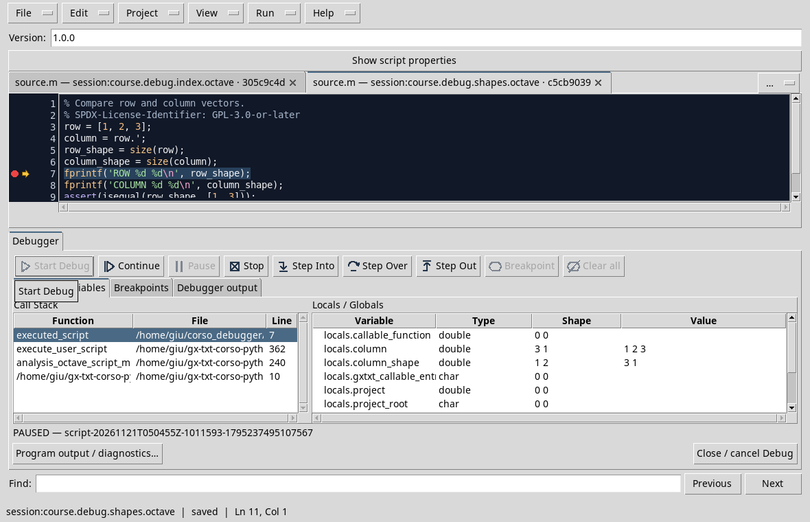
This screen, taken from the exercise on the forms, shows where to read type, shape and value of the vectors. In the fit also compares the dimensions of x, y and prediction before subtracting. The arrangement requires a maximum residual less than 1e-10: the arithmetic in mobile comma can leave very small differences, therefore it is not necessary to demand an exact zero.
Exercise
If the maximum residual is 1e-14, exceeds 1e-10 tolerance?
Worked solution
No. It is smaller than tolerance; the rounded six decimal print can show zero even when the internal value is not exactly zero.
D52 — Numerical integration and scale
Integration and unity must be consistent: a formula can be performed without errors and produce a result thousand times too large if time is expressed in the wrong drive.
Time, speed and distance
In integral.m, time_s = [0, 1, 2, 3] is expressed in seconds and speed_m_per_s = [2, 2, 2, 2] in meters per second. The area under the curve is 2 × 3 = 6 meters. Import and record the script in Octave Scripts, put a breakpoint on the print and start the debugger. Check the vectors and distance_m, then continue: the press is DISTANCE 6.0 m.
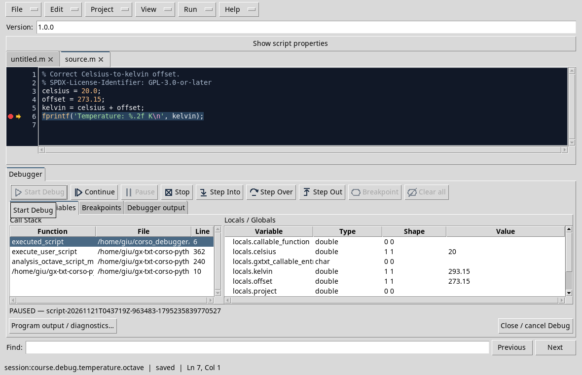
The image resumes the conversion of the D40: the debugger shows numbers, while the names and context clarify the units. If time came as [0, 1000, 2000, 3000] milliseconds, convert it into seconds by splitting to 1000 before trapz. Pass it directly to the formula with speed in m/s would produce 6000, without correctly representing meters.
Exercise
What distance runs through a constant speed of 2 m/s in 3 s?
Worked solution
6 m. The product between seconds and meters per second leaves meters.
D53 — From Dataset to plot
A correct chart requires both correct values and the right association between sizes and axes. Before you build it, stop by reading the Dataset.
From Session to Axes
Follow the D41 to create a debug_sensor_series test session, then the D39 to read time_s and voltage_v. The data are [0, 1, 2] s and [1, 2, 3] V respectively. The Dataset is created-only: to repeat the publication choose a new session or a new ID and update it also in the reading script.
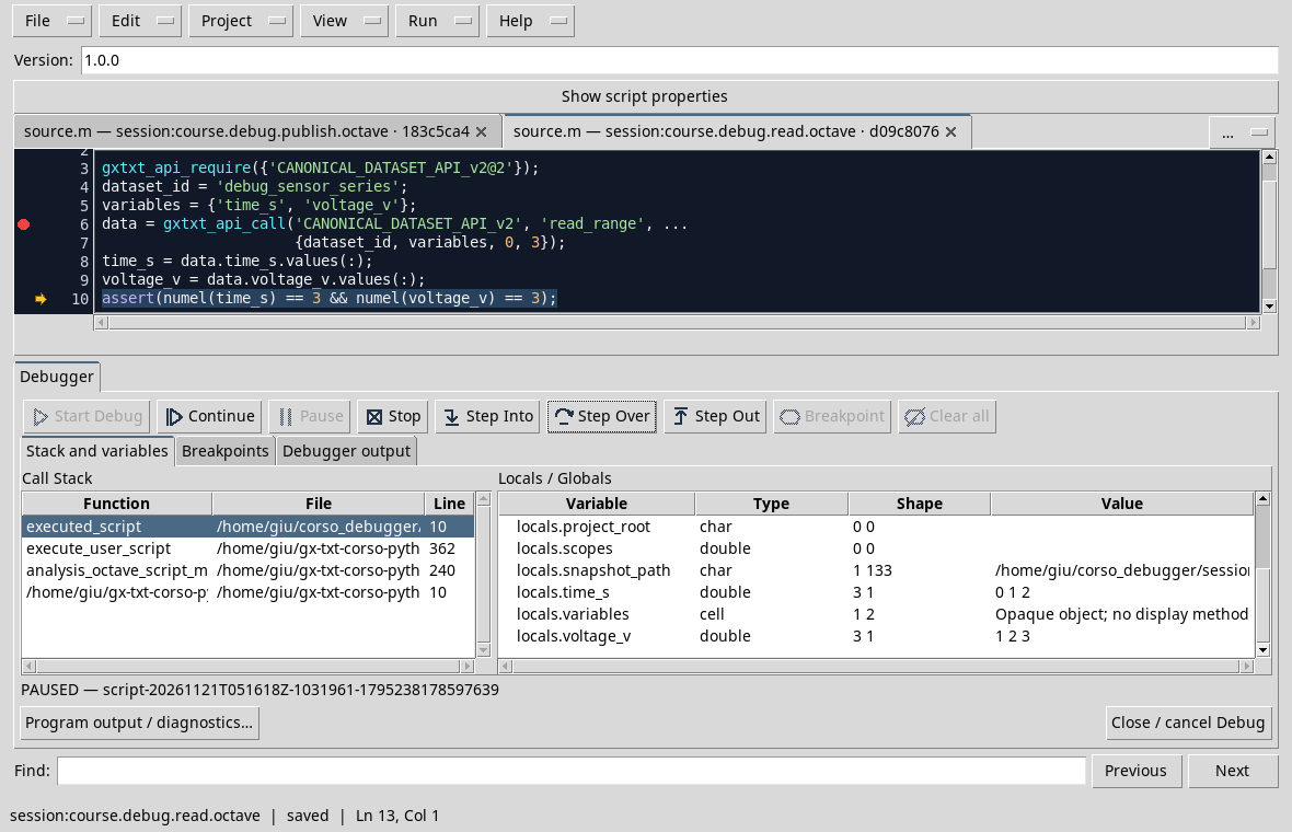
In the D39 screen, we control values and shapes after read_range. To prepare an XY chart combines time with horizontal axis and vertical tension; the expected pairs are (0, 1), (1, 2), (2, 3). Reverse the variables preserves three numerical pairs but changes the meaning of the chart. It carries units and names on the axes and checks a known point before drawing conclusions.
The sensor_plot.m script builds the chart through Plot Dataset API. Import it to the same Session, save it and start the debug; after the eventual initial break, press Continue. In the test the Job is finished with COMPLETED and produced the following chart with the native renderingr. The file is the result exported by GX-TXT, not a viewer screen.
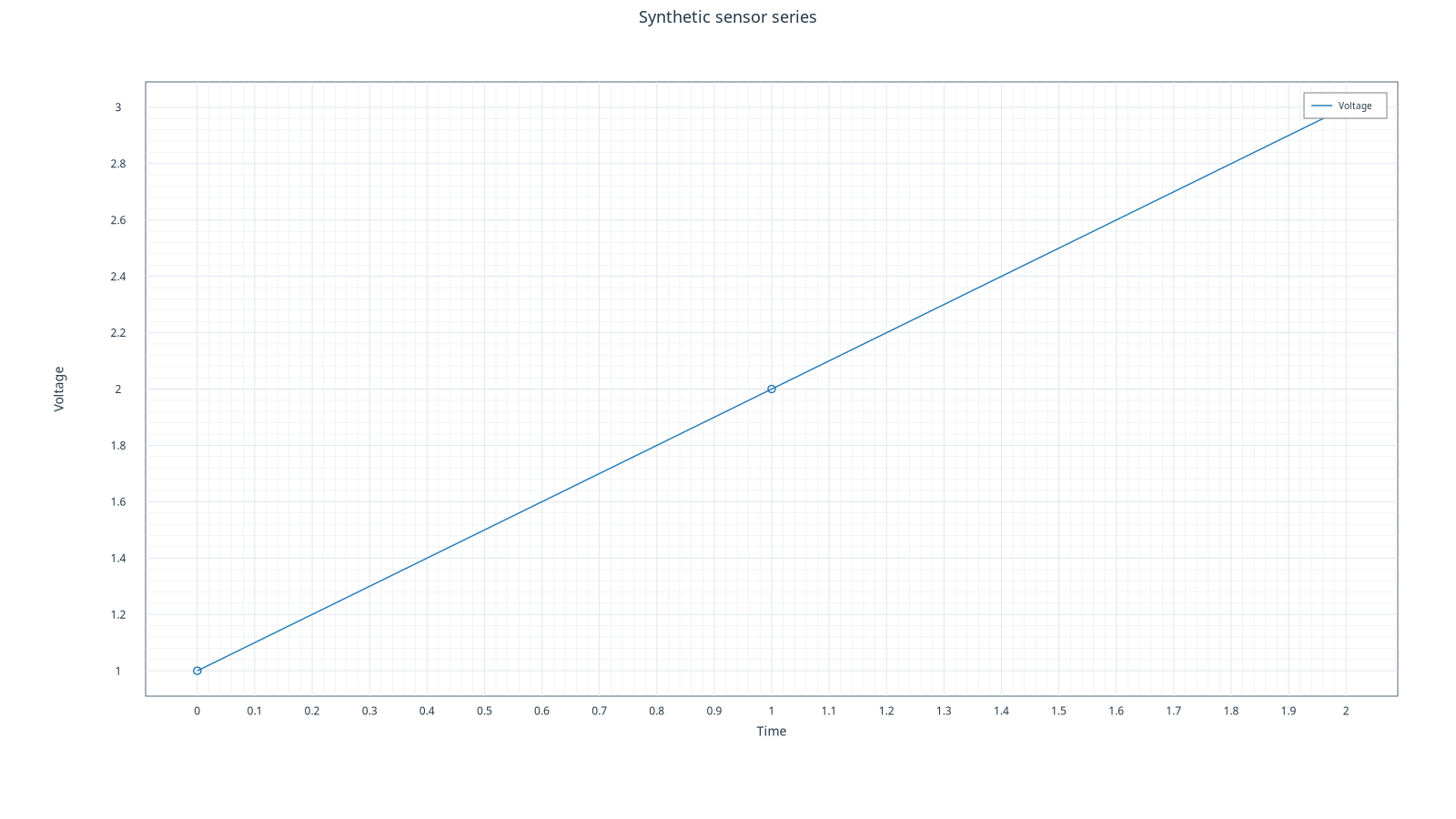
The graph uses the Time and Voltage names; in the documentation it explicitly associates the s and V units. The availability of the API and the renderr depends on the installed configuration.
Exercise
What do you get with 1 s time and 2 V voltage?
Worked solution
With time on X and voltage on Y the point is (1, 2); reverse the axes would give (2, 1) and a different interpretation.
D54 — A multifile project with a propagated error
When a data crosses multiple functions and files, the point where an unexpected result appears does not necessarily coincide with its origin. We follow the value from the caller to the support function.
A reproducible base
Prepare the main.py and helpers.py project, as in the D18. The caller passes 4 and expects adjust to return 5. Save both files and stop the debugger on the calculation line in the helper.
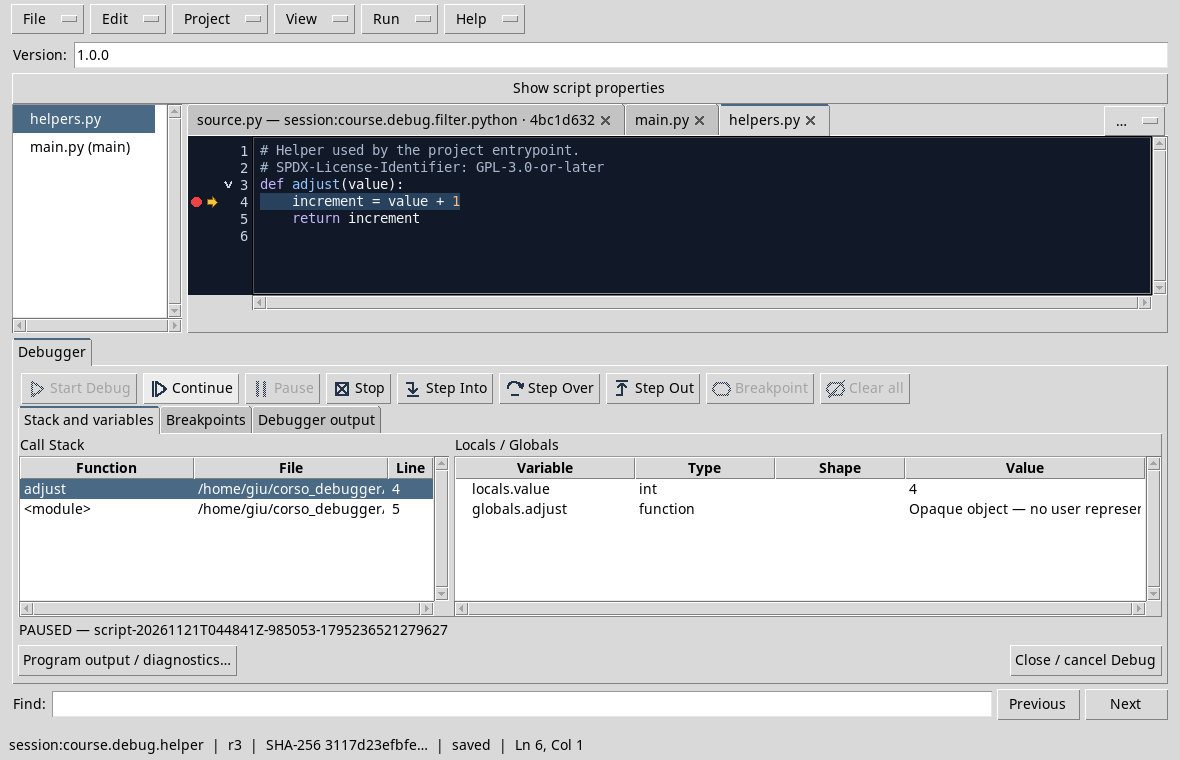
The test shows value = 4 in the function and caller in the stack. If a copy of the helper incorrectly added 2, the symptom in the caller would be 6, but the point to be corrected would be the operation in the helper. To practice, change a copy of the project, save and restart: first check the incoming argument, then the operation and finally the returned value. Update or temporarily remove the intentionally unsatisfied statement during diagnosis and restore it to check the correction.
Exercise
If the helper already receives 5 instead of 4, is it enough to correct his addition?
Worked solution
Not necessarily: you first need to go back to the caller and check why he provided 5. The value observed at the entrance distinguishes a problem upstream from one in the function.
These cases prepare the final project, in which it is necessary to document the defect, correction and verification so that another person can repeat them.
Previous: Module 08 · 10-module course contents · Next: Module 10
Other steps of this project
- Debugging GNU Octave in GX-TXT: Breakpoints, Variables and Public APIs
- GX-TXT Debugger · Module 08 — Projects, revisions and Sessions
- GX-TXT Debugger · Module 10 — Independent debugging and the final project
- GX-TXT Debugger · Guide 05 — Debugging scientific data: vectors, structures and Datasets
- GX-TXT Debugger · Guide 06 — Debugging a complete scientific workflow
- GX-TXT Debugger · Module 01 — Foundations and the first Debug Job