

OpenFOAM 14 Part 4: controlDict and Simulation Control
Part 4 of 8 of the case-building series in Learning OpenFOAM 14. Part 3 defined the initial fields and boundary conditions of the channel; this part moves to the layer that decides when the case starts, how it advances and when it writes results: the system/controlDict file.
The task. Read and write system/controlDict for OpenFOAM Foundation 14: solver module selection, start and stop rules, simulated time, output policies, restart and monitored execution.
The result. A complete reference controlDict, the ability to predict steps, write times and directory names before running, and a safe method for resuming or stopping a calculation.
Simulated time != CPU time
10 steps are calculated; output is written at steps 5 and 10. Settings: deltaT = 0.002 s | writeControl = timeStep | writeInterval = 5. The full timeline is in Figure 1, section 4.
How to use this part
Prerequisites. This part assumes the seven-step CFD workflow of the first worked case (laminar channel flow and Poiseuille validation) and the preceding parts on case structure (Part 1), mesh (Part 2) and fields (Part 3).
Scope. OpenFOAM Foundation 14. Read and write system/controlDict; reason about solver selection, start/stop rules, simulated time, output policies, restart, and monitored execution.
Reading path
Main track: solver selection → time control → output scheduling → restart → adaptive stepping → safe experiments. The Optional refresher boxes can be skipped by readers already fluent in CFD.
Reference case: 3D laminar rectangular channel | Official guide: doc.cfd.direct/openfoam/user-guide-v14.
Learning contract
This unit does not build a new mesh and does not prescribe new boundary conditions. It teaches the layer that controls when a case begins, how its progress is measured, and when results are written.
You should already have
- OpenFOAM Foundation 14 enabled in a shell (
foamVersion). - The channel mesh and field files from Parts 2–3, or an equivalent completed v14 tutorial case.
- An independent, editable copy of the case; never modify the reference case.
- Working
system/fvSchemes,system/fvSolution, and physics files if an actual solver run is planned.
At the end of this part, you should be able to
- Select the solver module used by
foamRunin OpenFOAM 14. - Predict start time, stopping condition and output directory names.
- Explain the difference between
timeStep,runTimeandadjustableRunTimeoutput. - Perform a restart without confusing the initial
0/directory with a saved later time. - Inspect time controls and logs before altering a live calculation.
Not in this unit
Which spatial discretisation to use belongs to Part 5. Linear solver tolerances and SIMPLE/PIMPLE corrections belong to Part 6. Valid CFD physics and boundary conditions cannot be fixed by changing controlDict.
Reading map
| Sections | Topic | Proof of understanding |
|---|---|---|
| 1–3 | Dictionary and time semantics | Identify the controls that advance the run |
| 4–7 | Write settings, safety, restart, adaptive stepping | Predict files and resumed states |
| 8–11 | Run-time changes and laboratory | Perform a controlled A/B comparison |
| 12–14 + appendix | Exercises, diagnosis, references | Explain and rebuild the settings |
1. What is controlDict?
The file system/controlDict configures the OpenFOAM time database and run-wide input/output controls. It is not the place where velocity boundary conditions or the finite-volume schemes are defined.
| Directory | Content |
|---|---|
0/ | fields / initial and boundary data |
constant/ | mesh / physical models |
system/ | simulation and numerical controls |
OpenFOAM Foundation 14: a solver module
In v14, the normal single-region workflow uses the foamRun application. The solver entry in controlDict selects a loadable solver module. This differs from many older tutorials that used an application simpleFoam; or application icoFoam; entry.
V14 structural excerpt:
FoamFile
{
    format      ascii;
    class       dictionary;
    location    "system";
    object      controlDict;
}
solver          incompressibleFluid;
Scope of the exampleincompressibleFluid is appropriate as an illustration of module selection, not a guarantee that a case is runnable: mesh, fields, properties and numerical dictionaries must also be compatible.
Read the entry, not just the filename
A historical tutorial can be useful conceptually while still containing version-specific syntax. If the configured module and application disagree with the intended v14 workflow, inspect a native v14 example first.
Deep dive: the time database (runTime)
Every OpenFOAM application builds a Time object at start-up (usually called runTime in the code). It is at once the clock of the calculation and the root registry of every object that can be read or written: mesh, fields, dictionaries. When a field is “written”, it is really runTime that decides whether the current instant is a write time and asks every registered object with automatic writing enabled to save itself in the current time directory.
This is why controlDict is read before any other case file: without it there is no database for the other objects to attach to. Even a utility that does not advance in time, such as blockMesh, needs a readable controlDict (as seen in Part 2). The numerically named directories (0, 0.01, …) are the “snapshots” of the database; after a solver write, each also contains a uniform/ subdirectory with a time file that records the time value, the step index and the current time step (see section 6).
The installation-wide settings (units, OptimisationSwitches, DebugSwitches) are not in the case controlDict but in $FOAM_ETC/configDict; they can be overridden for a single case by copying the sample with foamGet configDict into the system directory (User Guide §4.3).
Deep dive: how foamRun loads a module, and the mapping from old solvers
foamRun is a generic application: it reads the solver keyword, loads the shared library of the module with that name, and then runs a common time loop that calls the module’s functions at each step (momentum predictor, pressure corrector, transport and thermophysical models). Physics and algorithm live in the module; time control, writing and function objects remain in foamRun and in the time database. Multi-region cases (for example fluid + solid) use foamMultiRun, with the modules given per region in regionSolvers.
| Old application | Foundation module (with foamRun) |
|---|---|
icoFoam, simpleFoam, pimpleFoam | incompressibleFluid |
interFoam | incompressibleVoF |
rhoSimpleFoam, rhoPimpleFoam, buoyantFoam | fluid |
chtMultiRegionFoam | foamMultiRun with fluid and solid regions |
The table is an orientation, not an exhaustive list: the authoritative list for your installation comes from the commands below. Steady versus transient is no longer chosen by changing application: with incompressibleFluid it is decided by the ddtSchemes entry in fvSchemes (steadyState or, for example, Euler), the subject of Part 5.
foamToC -solvers                 # solver modules known to this installation
foamInfo incompressibleFluid     # description and example tutorials
foamDictionary -entry solver -value system/controlDict
Typical error: a controlDict copied from an old tutorial with application simpleFoam; and no solver makes foamRun fail with a FOAM FATAL IO ERROR of the form “keyword solver is undefined in dictionary …/system/controlDict”. A misspelt module name instead produces a selection error that names the unknown type. Some Foundation tutorials also contain an application foamRun; line: tutorial scripts use it to know which executable to launch, but the entry that decides the physics remains solver.
2. A complete reference controlDict
This teaching configuration uses a fixed numerical time step so that output times are easy to predict. It is deliberately conservative in file retention: nothing is automatically purged.
Teaching example — system/controlDict:
FoamFile
{
    format          ascii;
    class           dictionary;
    location        "system";
    object          controlDict;
}

solver              incompressibleFluid;

startFrom           startTime;
startTime           0;
stopAt              endTime;
endTime             0.020;
deltaT              0.002;

writeControl        timeStep;
writeInterval       5;
purgeWrite          0;
writeFormat         ascii;
writePrecision      8;
writeCompression    off;
timeFormat          general;
timePrecision       6;

runTimeModifiable   yes;
adjustTimeStep      no;
For a compatible transient case, this configuration plans 10 steps from 0 to 0.020 and regular writes at steps 5 and 10, i.e. at simulated times 0.010 and 0.020. Whether a particular simulation advances normally depends on the solver and the other case files.
The critical distinction
Fixed time step is chosen here to teach the time database. A solver using steadyState discretisation may treat the reported time as an iteration counter instead of physical seconds; do not interpret it as laboratory time.
A note on names: with timeFormat general; the written directories will not be called 0.010 and 0.020 but 0.01 and 0.02, because the general format drops trailing zeros (section 5). The time is the same; only its representation as a directory name changes.
Deep dive: every entry, its role and its default
The v14 User Guide (§4.4) lists the time-control entries and the writeControl/writeInterval pair as mandatory; the others have defaults. Writing them explicitly anyway makes the file self-documenting and protects against future changes of defaults.
| Entry | Value here | Role | Default / notes |
|---|---|---|---|
solver | incompressibleFluid | module loaded by foamRun | none: required by foamRun |
startFrom | startTime | which state to read | see section 3 |
startTime | 0 | time read with startFrom startTime | ignored with latestTime/firstTime |
stopAt | endTime | stop rule | see section 3 |
endTime | 0.020 | final time | used with stopAt endTime |
deltaT | 0.002 | time step (or iteration increment) | initial value if stepping is adaptive |
writeControl | timeStep | how the write interval is measured | mandatory |
writeInterval | 5 | write interval | mandatory; unit depends on writeControl |
purgeWrite | 0 | maximum number of times kept | 0 = no purging |
writeFormat | ascii | field format | ascii |
writePrecision | 8 | significant digits in ASCII | 6 |
writeCompression | off | gzip compression | off |
timeFormat | general | directory-name format | general |
timePrecision | 6 | digits of directory names | 6 |
runTimeModifiable | yes | re-reading dictionaries during the run | see section 8 |
adjustTimeStep | no | adaptive stepping | no |
To see the file as OpenFOAM reads it, with macros expanded and effective values, use foamDictionary -expand system/controlDict. The guide also lists less common entries: libs (additional libraries to load), functions (section 9), graphFormat (graph data format: raw by default, gnuplot, csv, vtk, ensight) and beginTime (section 4).
Deep dive: when “time” is only an iteration counter
In a steady calculation the time derivative is removed from the equations (ddtSchemes { default steadyState; }) and the module uses a SIMPLE-type algorithm. The time database still advances, however: every “step” is one under-relaxed iteration towards the steady solution. By convention deltaT 1; is used, so time equals the iteration count.
The backward-facing step tutorial of the v14 User Guide (§2.1.7 and §2.1.9) shows this well: endTime 2000, deltaT 1, writeControl timeStep, writeInterval 100. The run stops earlier, when the initial residuals drop below the residualControl tolerances in fvSolution: the log reports SIMPLE convergence in 285 iterations and the directories 100, 200 and 285 are written. The last is not a multiple of 100: when stopping on convergence the module writes the final state.
Practical consequence: in a steady case a directory name such as 285 does not mean “285 seconds”, and a deltaT other than 1 does not change the converged solution; it only changes the names. Before interpreting a time directory, therefore, check ddtSchemes with foamDictionary -entry ddtSchemes system/fvSchemes.
3. Starting, advancing and stopping
Start time selection
| Entry | Meaning | Typical use |
|---|---|---|
startFrom firstTime; | Read the earliest available time directory. | Read a case from its earliest saved state. |
startFrom startTime; | Use the time selected by startTime. | A deliberate fresh start from 0. |
startFrom latestTime; | Read the latest available time directory. | Resume from a previously written result. |
Stop conditions
| Entry | What it does |
|---|---|
stopAt endTime; | Advance until the configured endTime condition is met. |
stopAt nextWrite; | Stop at the next scheduled write event; useful for an orderly interruption. |
stopAt writeNow; | Stop after the current time step and write fields. |
stopAt noWriteNow; | Stop after the current time step without an additional write. |
Example: a deliberate start and target
startFrom       startTime;
startTime       0;
stopAt          endTime;
endTime         0.020;
deltaT          0.002;
Optional refresher · What is a time step?
For a transient flow, advancing by one time step updates the estimated state from t to t + Δt. A time step is not identical to one linear-solver iteration: an algorithm may perform several algebraic solves and corrections during a single time step.
Deep dive: how OpenFOAM decides it has reached endTime
The planned number of fixed steps is N = (endTime − startTime)/Δt; in the example 0.020/0.002 = 10. The comparison is not done in exact arithmetic, though: 0.002 is not exactly representable in binary floating point and ten successive sums do not give exactly 0.02. To avoid an extra or missing step caused by round-off, the Foundation time database keeps running while the current time is less than endTime − ½Δt, and the directory name is generated with timePrecision digits.
Numerical example: with endTime 0.021 and Δt = 0.002 the criterion is t < 0.020. After the tenth step t = 0.020, so the run stops at 0.020, not 0.021: with a fixed step there is no “shortened” final step. If endTime is not a multiple of Δt, the actual final time is the nearest multiple according to this criterion. Always predict it and compare with the last Time = line of the log.
With stopAt writeNow and noWriteNow the time database, at the first re-read of the file, effectively sets the end at the current step; with nextWrite it waits until the current step is also a write time. With firstTime and latestTime the value of startTime does not matter; with startTime a directory with that time, containing the required fields, must exist.
Deep dive: what happens inside one time step
With incompressibleFluid in transient mode the algorithm is PIMPLE. One time step contains nOuterCorrectors outer loops; each has an (optional) momentum predictor, i.e. one linear-system solve per velocity component, followed by nCorrectors pressure corrections, each solving a Poisson equation for p (plus any non-orthogonal corrections). With 1 outer loop and 2 correctors, up to 3 velocity systems and 2 pressure systems are solved per step, and each system needs several linear-solver iterations of its own.
In the log this appears as one block per step: a Time = … line, then lines of the form “solver: Solving for Ux, Initial residual = …, Final residual = …, No Iterations …” for each solve, the continuity errors and finally ExecutionTime and ClockTime. Counting Time = lines counts steps; counting “Solving for p” lines counts pressure solves. PIMPLE settings and tolerances belong to fvSolution and are covered in Part 6.
4. Simulated time and write scheduling
Use the exact same deltaT = 0.002 and endTime = 0.020 in all examples below. Only the writing policy changes. The timeline is based on a transient run with ten completed time steps.
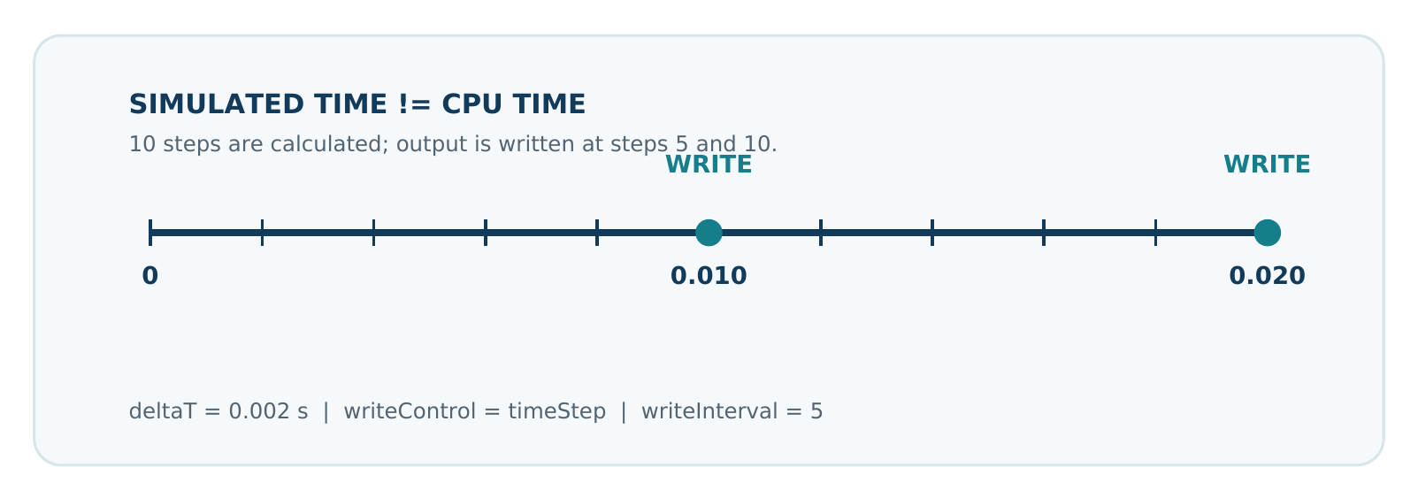
Three policies you must not confuse
| Control pair | Interpretation | Expected written times |
|---|---|---|
timeStepwriteInterval 5; | Write every five numerical steps. | 0.010, 0.020 |
runTimewriteInterval 0.006; | Request output at 0.006-s simulated-time intervals; here the grid of steps aligns. | 0.006, 0.012, 0.018 |
adjustableRunTimewriteInterval 0.006; | Write on scheduled simulated times; adjust step size to hit a write boundary when needed. | 0.006, 0.012, 0.018 |
Important: runTime is not wall clock
In writeControl, runTime refers to simulated time. For output based on real elapsed execution time, v14 provides clockTime; cpuTime refers to processor time.
The values in the table are scheduled regular writes, not a guarantee of an extra write exactly at the termination time. Depending on the stop mode, the final state might not correspond to a scheduled output.
Deep dive: how a write time is decided
timeStep. The current step is a write time when its index is an integer multiple of writeInterval (which must therefore be read as a whole number of steps). The index is the one held by the time database: after a restart it continues from the value saved in uniform/time; it does not restart from zero.
runTime / adjustableRunTime. At each step a write index is computed as the integer part of (t − tref + ½Δt)/writeInterval; when this index increases relative to the last write, the current step becomes a write time. The half step makes the comparison robust to round-off: with Δt = 0.002 and interval 0.006, at t = 0.006 one gets (0.006 + 0.001)/0.006 ≈ 1.17 → index 1 → write. If the interval is not a multiple of Δt, the write lands on the step nearest to the requested instant (within half a step), not on the exact instant, and the written times are not evenly spaced.
The reference tref matters after a restart. The v14 Guide documents the optional beginTime entry, which anchors write times to multiples of writeInterval from that time, for cases with an awkward start time. After a restart from a time that is not a multiple of the interval, check where the first write falls with foamListTimes instead of assuming it.
clockTime / cpuTime. The interval is in seconds of real or CPU time; the simulated times written depend on the machine load and change from one execution to the next. They are useful as safety checkpoints on long runs (for example writeInterval 3600 with clockTime), never for a reproducible comparison.
Deep dive: how adjustableRunTime adjusts the step
With adjustableRunTime the time database, whenever the step is set, computes the time remaining to the next write and divides it into a whole number of equal steps, rounding the ratio of remaining time to current step upwards. The new step is the remaining time divided by that number; the change relative to the previous step is bounded so as not to introduce abrupt jumps. The result is that writes land exactly on multiples of writeInterval.
Example: current step 0.004 s, next write due in 0.006 s. The ratio is 1.5 → 2 steps → Δt = 0.003 s. Without adjustment, with runTime, the steps would fall at 0.004 and 0.008 and the write “at 0.006” would end up at 0.008 (the nearest step within half a step, according to the rule in the previous note).
The v14 Guide recommends adjustableRunTime together with automatic stepping (adjustTimeStep yes): that is where it really matters, because the step changes continuously and without adjustment the written times would be arbitrary, as the dam-break tutorial (§2.2) notes. With a fixed step already aligned with the interval, as in the table example, runTime and adjustableRunTime give the same times.
5. Output formats, directory names and retention
A simulation can run correctly but leave an impractical number of files, or too few results for analysis. Treat output as part of the experimental design.
| Setting | Effect |
|---|---|
writeFormat ascii/binary | Readable text versus compact binary field format. |
writePrecision | Numerical precision of written ASCII values; not solver accuracy. |
writeCompression on/off | Compression of output files on disk. |
timeFormat | Formatting of output time directory names. |
timePrecision | Digits used for time-directory names; distinct from field-value precision. |
purgeWrite | Maximum number of retained written time directories when enabled. |
Understand purgeWrite before using it
Do not enable purging in the teaching master:
purgeWrite      0;     // Do not purge saved time directories.

// Separate example: retain only a rolling set
// purgeWrite   2;
Data-loss warningpurgeWrite 2; removes older written time directories as new ones are produced. It is unsuitable when the complete transient history is required for validation, comparisons, or reproducibility. Work only on a copy; changing the setting is not reversible.
Time-directory naming
With timeFormat general; and sufficient timePrecision, directory names can represent times such as 0.01. Too little time precision can cause collisions or ambiguity; it does not change physical time-step accuracy.
Deep dive: ASCII, binary, precision and disk size
In memory OpenFOAM works in double precision (about 15–17 significant digits). In ASCII each value is written with writePrecision significant digits: with 6 (the default) a value such as 0.0123456789 becomes 0.0123457. The solver loses no accuracy during the run, but a restart from an ASCII directory starts from rounded values: for small variations or for bit-wise comparisons between a continuous and a resumed run, this is enough to make the histories diverge slightly. That is why the reference uses 8, and for rigorous restarts binary, which keeps every bit, is preferable.
With writeFormat binary the FoamFile header stays textual (with format binary;) but non-uniform value lists become raw bytes; less shows unreadable characters. With writeCompression on the files become U.gz, p.gz, etc.; OpenFOAM reads them transparently and zcat 0.01/U.gz | head -n 30 shows their beginning if they are ASCII.
Order-of-magnitude estimate for the Part 2 channel (40 × 10 × 5 = 2,000 cells; 5,350 internal faces): U holds 2,000 vectors, i.e. 6,000 numbers; in binary 8 bytes each ≈ 48 kB, in ASCII with 8 digits about 12–15 characters per number ≈ 70–90 kB. phi (one value per internal face) and p add similar amounts. Multiply by the number of writes: 1,000 writes of a 10-million-cell mesh are already hundreds of gigabytes. Always measure with du -sh instead of guessing.
Deep dive: timeFormat, timePrecision and name collisions
timeFormat accepts fixed, scientific and general (default). According to the v14 Guide, general uses scientific notation when the exponent is below −4 or at least timePrecision, otherwise decimal notation without trailing zeros. timePrecision (default 6) is the number of digits used.
| Time | general, 6 | fixed, 3 | Remark |
|---|---|---|---|
| 0,010 | 0.01 | 0.010 | same time, different name |
| 0,0125 | 0.0125 | 0.013 | fixed with 3 digits rounds |
| 0,00001 | 1e-05 | 0.000 | with fixed, 3 digits: collision with 0 |
A collision is serious: two different instants would write into the same directory, overwriting each other, or a positive time would be confused with 0. The Foundation time database detects the situation when the step is too small for the available digits, automatically increases timePrecision and reports it with a warning in the log (“Increased the timePrecision …”). Do not rely on this mechanism: choose the precision according to the smallest expected step (with adaptive stepping, according to what appears in the log) and look for the warning in the log.
Deep dive: what purgeWrite actually deletes
The v14 Guide describes purgeWrite as a limit on the number of retained time directories: once the limit is exceeded, older directories are overwritten cyclically, i.e. deleted at every new write. With purgeWrite 2 and writes every 5 steps in the reference case extended to 0.040 s, only 0.035 and 0.04 would remain at the end; 0.01, 0.015, … would have been lost during the run.
In the Foundation implementation the queue of directories to delete holds the times written by the current execution: the initial 0/ directory and, after a restart, the directories produced by earlier executions do not enter it. Do not treat this as a guarantee, though: check on a copy with foamListTimes before and after.
Legitimate use: very long runs where only statistics collected by function objects (section 9) and a recent restart point matter. There is also the foamListTimes -rm tool, which deletes all listed time directories except 0: it too is irreversible and must only be used on copies, never as a diagnostic shortcut (section 13).
6. Restarting a case safely
A restart is a new execution that reads an existing written state. It is not the same as simply choosing a later endTime. A valid restart requires compatible saved fields, mesh and physical/numerical settings.
The minimal restart change
Restart after a saved 0.020 state:
startFrom       latestTime;
stopAt          endTime;
endTime         0.040;
For the illustration, the last available written time is 0.020. The next execution reads that state and continues toward 0.040; it does not go back to 0/U and 0/p. With latestTime, the startTime value is not the selector.
Safe sequence
Example shell workflow:
# Work in a personal case directory; save an exact copy.
cp -a channelCase channelCase_restart
cd channelCase_restart

foamDictionary -entry startFrom -value system/controlDict
foamDictionary -entry endTime -value system/controlDict
ls -d [0-9]* 2>/dev/null          # Inspect, do not infer.

# After editing controlDict and checking other case files:
foamRun > log.restart 2>&1
less log.restart
Preserve evidence
Always keep the original case and a full record of the settings used for the first run. If mesh or model assumptions change, the saved fields may no longer be a consistent restart state. A copied case is safer than editing or deleting old time directories.
Three questions before restart
- Which time directory will actually be selected?
- Do its fields match the active mesh and model?
- Are the requested new stop time and output schedule consistent with that starting state?
Deep dive: what a time directory contains and what the restart reads
After a solver write, a directory such as 0.02/ contains the solved fields (U, p), the face flux phi (with incompressibleFluid; on restart it is read if present instead of being rebuilt from velocity) and any model fields (for example nut, k, omega with a turbulence model). The uniform/ subdirectory holds the time file with the time value, the name, the step index and the latest time steps (deltaT, deltaT0).
foamDictionary 0.02/uniform/time
# typical entries: value, name, index, deltaT, deltaT0
foamDictionary -entry index -value 0.02/uniform/time
Two consequences. First: with writeControl timeStep the index continues, so a restart from 0.02 (index 10) with writeInterval 5 writes at 0.03 and 0.04 (indices 15 and 20), consistently with the first run. Second: the time database uses the information in uniform/time to resume; if you changed deltaT in controlDict for the restart, check in the log the step actually used in the first steps (for example the interval between two Time = lines) rather than assuming it.
Deep dive: tools for preparing a restart (and a trap)
foamListTimes (Guide §4.7) lists the time directories excluding 0; with -latestTime it shows only the one that startFrom latestTime will select. foamDictionary -set edits entries repeatably and accepts several assignments in one call with comma-separated key=value syntax; after every change read the value back with -value.
# Predict what latestTime will select, without running anything
foamListTimes -latestTime

# Edit entries reproducibly instead of by hand
foamDictionary -set "startFrom=latestTime, endTime=0.040" system/controlDict
foamDictionary -entry startFrom -value system/controlDict
foamDictionary -entry endTime -value system/controlDict
The trap: foamCloneCase old new copies only 0, system and constant. It is perfect for a fresh start, but a clone does not contain the later time directories: a latestTime restart on the clone would silently start again from 0/. For a restart use cp -a, which copies everything while preserving dates and permissions, as in the safe sequence above.
If the mesh has changed (for example after refinement), the saved fields no longer have the right number of cells and reading fails. That is no longer a restart but a new calculation initialised from another: the v14 Guide (§5.8) describes mapFields for mapping fields between different geometries.
7. Adaptive time stepping and Courant number
For transient solvers that support automatic timestep adjustment, controlDict can express a target Courant-number limit. This is a numerical control, not an alternative to selecting appropriate mesh resolution and models.
Optional refresher · Courant number
For one-dimensional advection on a uniform mesh, a useful estimate is Co ≈ |U| Δt / Δx. At |U| = 0.05 m/s, Δt = 0.002 s and Δx = 0.001 m, Co ≈ 0.10. In practical 3D finite-volume calculations, the reported local/max Courant numbers depend on face fluxes and cell volumes.
V14 transient example — check module support:
adjustTimeStep      yes;
maxCo               0.5;
maxDeltaT           0.005;

writeControl        adjustableRunTime;
writeInterval       0.010;
What changes?
- The solver can change
deltaTduring the run when its time-control implementation supports these entries. maxCoexpresses a target upper Courant number; it does not certify stability or solution accuracy.maxDeltaTimposes an additional configured timestep ceiling when supported.adjustableRunTimecoordinates scheduled output with automatically changing timesteps.
Fixed-step baseline first
Keep adjustTimeStep no; in the first controlled experiments. Change to adaptive stepping only after confirming that the selected v14 module and case numerics support it, and inspect the solver log for the actual timestep history.
Deep dive: the Courant number as OpenFOAM computes it
In finite volumes velocity is not carried by a single |U| but by the volumetric face fluxes φf = Uf·Sf (m³/s). For each cell P OpenFOAM computes CoP = ½ Δt Σf |φf| / VP: the sum of all incoming and outgoing fluxes, halved (what enters equals what leaves), relative to the volume. In words: the fraction of the cell volume swept by the fluid in one step. The log reports a “Courant Number mean: … max: …” line for each step, i.e. the cell average and the maximum.
For a uniform hexahedron with flow only along x the formula reduces to |U|Δt/Δx, i.e. the refresher’s estimate. Example on the Part 2 channel (Δx = 2.5 mm, Δy = Δz = 1 mm) with axial velocity 0.05 m/s and Δt = 0.002 s: Co = 0.05 × 0.002 / 0.0025 = 0.04. If the mesh is refined in x to Δx = 1.25 mm the Courant number doubles to 0.08 at the same step: refining the mesh without reducing the step increases Co. Use the peak velocity, not the mean: in a duct the centreline maximum is noticeably higher than the mean velocity.
Stability and accuracy are different questions. OpenFOAM’s implicit time schemes can remain stable even with Co > 1, but the temporal discretisation error grows with Δt and pressure-velocity coupling algorithms with few correctors lose accuracy. For problems with interfaces (VoF) there is a separate limit, maxAlphaCo, used by the dam-break tutorial together with maxCo 1.
Deep dive: how the adaptive step grows and shrinks
In the Foundation implementation of the fluid modules the new step is obtained from the ratio r = maxCo/Comax between the target and the current maximum Courant number. When r < 1 (Courant too high) the step is reduced immediately in proportion; when r > 1 growth is damped (factor no larger than 1 + 0.1·r) and capped at a 20% increase per step. Finally the step never exceeds maxDeltaT. At start-up the controlDict deltaT is the initial value, reduced at once if it already violates maxCo.
Example with this section’s excerpt: initial Δt 0.002 s, Comax = 0.10, maxCo 0.5 → r = 5, but growth is capped at ×1.2 per step: 0.0024, 0.00288, 0.003456, 0.004147, 0.004977; the next step (0.00597) is then cut by maxDeltaT 0.005. With the step at 0.005 the expected Courant number is 0.10 × 0.005/0.002 = 0.25, still below 0.5: here the active limit is maxDeltaT, not maxCo. At the same time adjustableRunTime shortens the steps near 0.010 and 0.020 so that the writes land there.
Check in the log: with adaptive stepping a deltaT = … line appears at each step next to the Courant line. Extract the history with grep '^deltaT' log.foamRun and grep 'Courant Number' log.foamRun; if deltaT never changes despite adjustTimeStep yes, the module or the case is not using adaptation (for example because the case is steady).
8. Runtime changes and orderly stops
With runTimeModifiable yes;, OpenFOAM can re-read certain configuration data while a run is active. Not every dictionary entry can be changed safely or takes effect in the same way. Never assume that changing an arbitrary file updates the running physical model.
Controlled run and inspection
Run monitoring:
# Run in a terminal and capture the output.
foamRun > log.foamRun 2>&1

# In a second terminal while it runs:
tail -f log.foamRun
A useful log usually contains time/iteration information, solver residuals, execution time, and occasionally a Courant number. The specific messages depend on the solver module and settings.
Request a clean stop
Orderly stop at the next scheduled output:
// While a run is active, in system/controlDict:
runTimeModifiable   yes;
stopAt              nextWrite;
When the running application honours the re-read, it should complete the next scheduled write before stopping. If you must interrupt immediately, distinguish a process interruption from an orderly configured stop; the last valid written fields are the restart point.
Server practice
For shared laboratory servers: inspect disk space before frequent writes, redirect logs to files, and do not change a colleague’s running case. If the calculation is expensive, keep a dated copy of the control file and explicitly record every runtime modification.
What to record
Log the setting changed, its prior and new values, the simulation time when the change was requested, and the first log message confirming it took effect. Do not silently reinterpret a run as having constant settings.
Deep dive: how re-reading works and how to edit a file safely
At each step the dictionaries registered as “re-read if modified” are compared with the file on disk. The checking method is the fileModificationChecking option of the OptimisationSwitches in $FOAM_ETC/configDict (default timeStampMaster: modification-date check performed by the master process in parallel; alternatives timeStamp, inotify, inotifyMaster). On network file systems fileModificationSkew also matters: the seconds subtracted from the file date to compensate for delays and unsynchronised clocks (Guide §4.3). When a file is re-read, the log reports a message naming the re-read object (for example controlDict): that is the confirmation to record.
What responds reliably: the time and write controls of controlDict (endTime, stopAt, writeInterval, …) and, in general, the numerical parameters of fvSchemes and fvSolution. What must not be taken for granted: the mesh, the solver module (already loaded), the boundary conditions in the fields of the time directory in use, and many physical properties.
An editor that saves in several stages can make the solver read a half-written file, with a syntax error that stops the run. Safer: a single complete write with foamDictionary -set, preceded by a dated copy.
# 1. keep a dated copy of the file you are about to change
cp -p system/controlDict system/controlDict.$(date +%Y%m%d-%H%M%S)
# 2. change one entry in a single, complete write
foamDictionary -entry stopAt -set nextWrite system/controlDict
# 3. look for the confirmation in the log
grep -n 'controlDict' log.foamRun | tail -n 3
Deep dive: immediate interruptions, signals and what is lost
Ctrl-C (SIGINT) or kill terminate the process without writing: everything computed after the last write is lost and the restart point is the last complete directory. An interruption during a write can leave an incomplete time directory (some fields missing or truncated): before a latestTime restart check that the last directory contains all fields and, if not, move it out of the case rather than deleting it.
Comparing the orderly routes: stopAt writeNow writes immediately at the step after the re-read (no computation lost, but the written time is off the planned grid); stopAt nextWrite keeps the write grid (at the cost of waiting until the next event); stopAt noWriteNow stops without writing and is useful only when the data after the last write are not needed. There are also the OptimisationSwitches writeNowSignal and stopAtWriteNowSignal (Guide §4.3), which associate an operating-system signal with “write now” or “write and stop”; check their value in $FOAM_ETC/configDict with foamDictionary -entry OptimisationSwitches/writeNowSignal $FOAM_ETC/configDict before relying on them.
Template entry for the lab record: “2026-10-16 14:32 — case channel_B — endTime 0.020 → 0.040 — requested at t ≈ 0.014 — confirmed in the log at line N (controlDict re-read) — reason: extending the transient”.
9. Function objects: a preview
The optional functions dictionary in controlDict can request additional calculations during a run: sampling, probes, integrals or derived fields. These are data acquisition and post-processing controls, not replacements for fvSchemes or fvSolution.
Minimal placeholder — no function objects active:
functions
{
    // Function objects may be configured here.
}
What belongs to a function object?
| Question | Typical responsibility |
|---|---|
| What quantity is needed? | A sampled field, an average, a force, a flow rate, etc. |
| When should it be evaluated? | Its execution controls. |
| When should it be written? | Its writing controls, which may be distinct. |
| What name/file identifies the result? | Function object name and output options. |
How to learn the syntax independently
Documentation discovery:
foamInfo incompressibleFluid
foamInfo patchAverage

# Look at the working v14 tutorials before adding a
# particular function object to your own case.
echo "$FOAM_TUTORIALS"
The functions available depend on the OpenFOAM installation and libraries. Search native v14 tutorial cases for one suitable to the channel. Use the official function-object references in Chapter 7 of the guide (Post-processing) for complete syntax.
Do not overload this unit
This part introduces where function objects live and how to identify their purpose. The reference channel should first run correctly without any function objects; derived-output configuration can be added as a separate, testable step.
Deep dive: since v12, the system/functions file and #includeFunc
The v14 Guide (§7.2) states that since v12 function objects preferably go in a separate system/functions file, rather than in the functions sub-dictionary of controlDict: applications that do not use function objects then do not need to read them. The older location in controlDict, shown above, still works. Pre-configured functions are included with the #includeFunc directive, passing arguments in brackets; those with many parameters (for example forces) are copied into the case with foamGet and edited: a local copy in system takes precedence over the defaults in $FOAM_ETC/caseDicts/postProcessing.
# v12 and later: a separate system/functions file is preferred
foamGet functions                       # copies a template into system/
# inside system/functions, for example:
#includeFunc patchFlowRate(patch=outlet)

foamPostProcess -list                   # configured functions available
foamToC -functionObjects                # underlying function-object types
# after the run, with the models of the solver module constructed:
foamPostProcess -solver incompressibleFluid -func "patchFlowRate(patch=outlet)"
foamInfo gives a description and examples for models, modules and functions; foamPostProcess -list lists the configured functions available; foamToC -functionObjects lists the compiled function-object types. Results normally go in postProcessing/<name>/<start time>/. For the channel, an outlet flow rate (patchFlowRate) is the natural first check: it must equal the inlet flow rate imposed in Part 3.
Deep dive: execution and write controls of a function object
The table above separates “when to evaluate” from “when to write”. In Foundation function objects these two questions correspond to the executeControl/executeInterval and writeControl/writeInterval pairs, which accept the same modes seen in section 4 (timeStep, runTime, adjustableRunTime, clockTime, cpuTime) plus writeTime, which ties the event to the case field writes. A probe can thus be evaluated and written at every step (for a fine time history) while the full fields are saved only every 5 steps: this is precisely how to obtain a lot of data without filling the disk.
Watch consistency with purgeWrite: function-object data are not deleted by purgeWrite, but a function object run “after the fact” with foamPostProcess can only process the time directories that remain. Decide before the run which quantities are needed during execution and which can be derived afterwards.
10. Guided laboratory: baseline run
We reuse the same 3D channel with inlet, outlet, walls and previously defined 0/U and 0/p. Do not run until the remaining dictionaries and model files are valid for OpenFOAM Foundation 14.
Stage A — Inspect before changing
Read the existing configuration:
foamVersion
pwd
foamDictionary -entry solver -value system/controlDict
foamDictionary -entry startFrom -value system/controlDict
foamDictionary -entry writeControl -value system/controlDict
foamDictionary -entry writeInterval -value system/controlDict
Stage B — Set a predictable baseline
Values to set in your copy:
startFrom       startTime;
startTime       0;
stopAt          endTime;
endTime         0.020;
deltaT          0.002;
writeControl    timeStep;
writeInterval   5;
purgeWrite      0;
adjustTimeStep  no;
Stage C — Predict, then observe
- Predict how many steps will be completed and at which times output will be written.
- Inspect the initial directory list before the run; distinguish the original
0/from later result directories. - Run the existing v14 case with
foamRun; redirect its log. - Inspect the generated directories and compare them with your prediction.
- Record whether the run ended normally; do not infer successful completion just from the presence of a log file.
Run only a compatible complete case
The Part 3 fields and the Part 2 mesh are not sufficient by themselves to run a solver. For this laboratory use the already working tutorial case or the complete validated case supplied with the training series; avoid inventing missing physics or numerical files.
Deep dive: expected Stage C results and how to recognise a normal end
Prediction: 0.020/0.002 = 10 steps; writes at steps 5 and 10 → directories 0.01 and 0.02. Before the run ls shows 0, constant, system (plus any case scripts); afterwards 0.01, 0.02 and log.foamRun appear. 0/ remains unchanged: the solver does not overwrite it.
A normal end has three concordant signs: the last line of the log is End; no FOAM FATAL ERROR or FOAM FATAL IO ERROR appears in the log; the process exit code is 0 (echo $? right after foamRun). If | tee is used instead of redirection, the exit code is that of tee unless set -o pipefail is set first. A log file exists even after an error at the first step: that is why its mere presence proves nothing.
tail -n 3 log.foamRun              # a normal termination ends with the line "End"
grep -c '^Time = ' log.foamRun     # number of completed time steps (10 here)
grep -n 'FOAM FATAL' log.foamRun   # empty output = no fatal error recorded
foamListTimes                      # written times, 0 excluded
Deep dive: where to find a complete case for the laboratory
The two sources named are an already working native v14 tutorial or the complete validated case of the series: the first worked case, the laminar Poiseuille channel, contains all the files needed (mesh, fields, physicalProperties, momentumTransport, fvSchemes, fvSolution) for incompressibleFluid. Among the tutorials, look for those that select the same module and copy one into your working directory before touching it.
# Native v14 cases that select the incompressibleFluid module
grep -rl --include=controlDict 'incompressibleFluid' "$FOAM_TUTORIALS" | head
# Copy one to your own run directory before touching it
mkdir -p ~/run && cp -a "$FOAM_TUTORIALS/incompressibleFluid/cavity" ~/run/cavityBaseline
ls ~/run/cavityBaseline
The cavity path is the usual one in recent Foundation versions; if it differs in your installation, use the result of the grep search. Many tutorials need a mesh step (blockMesh) first or have an Allrun script: read it before running it and, for this laboratory, replace only the controlDict values of Stage B. A cavity is closed: its patches are not called inlet/outlet, but the time logic is identical.
11. Guided laboratory: compare writing strategies
Make separate copies of the validated baseline case so that output directories from the first experiment do not influence the second. Both cases should start from their own 0/ states.
Experiment A — Every 5 steps
writeControl    timeStep;
writeInterval   5;
Prediction: for Δt = 0.002 s and final time 0.020 s, scheduled regular output at 0.010 and 0.020.
Experiment B — Every 0.006 s
writeControl    runTime;
writeInterval   0.006;
Prediction: scheduled output at 0.006, 0.012 and 0.018 because every requested instant is an exact multiple of the fixed Δt. No regular event falls at 0.020.
Experiment C — Change only file format
writeFormat         binary;
writeCompression    on;
Run a third independent case copy and compare file size and readability, not flow physics. Remember that binary output is not intended for manual text inspection.
| Record in the lab sheet | Experiment A | Experiment B | Experiment C |
|---|---|---|---|
| Output directory names | ________ | ________ | ________ |
| Number of written snapshots | ________ | ________ | ________ |
| Elapsed execution time | ________ | ________ | ________ |
| Total results size | ________ | ________ | ________ |
Comparison rule
Never change time step, write cadence, physical fields and numerical solvers all at once. This exercise isolates one input/output decision at a time to support causal interpretation.
Deep dive: expected values for the sheet and how to measure them
| Sheet row | A | B | C |
|---|---|---|---|
| Directory names | 0.01, 0.02 | 0.006, 0.012, 0.018 | 0.01, 0.02 |
| Snapshots written (0 excluded) | 2 | 3 | 2 |
| Content of one directory | U, p, phi, uniform/ | as A | U.gz, p.gz, phi.gz, uniform/ |
| Execution time | reference | ≈ A (one more write) | ≈ A |
| Size | reference | ≈ 1,5 × A | smaller than A |
Two remarks to write on the sheet. In B the final state computed at 0.020 is not saved: the run performs 10 steps, but the last two (0.018 → 0.020) leave no trace on disk; a restart from B starts from 0.018. To avoid this, choose a writeInterval that divides the total interval. In C the size reduction depends on the mesh and the values (nearly uniform fields compress very well); on a 2,000-cell mesh the run time is dominated by start-up and the solver, so time differences of a few tenths of a second are noise: repeat the measurement before drawing conclusions.
# three independent copies of the same validated baseline
for c in A B C; do cp -a channelBaseline channel_$c; done

foamDictionary -set "writeControl=runTime, writeInterval=0.006" channel_B/system/controlDict
foamDictionary -set "writeFormat=binary, writeCompression=on" channel_C/system/controlDict

for c in A B C; do (cd channel_$c && foamRun > log.foamRun 2>&1); done

# measurements for the lab sheet
for c in A B C; do
  echo "== $c"
  (cd channel_$c && foamListTimes && du -sh $(foamListTimes) \
     && grep 'ExecutionTime' log.foamRun | tail -n 1)
done
12. Independent exercises
Exercise A — Read and classify (guided)
Given the complete reference controlDict in section 2, answer these questions without running the solver:
- Which entry chooses the v14 solver module? Which entry selects the starting state?
- How many time steps are planned, and when are the regular writes?
- Which entry governs time-directory name formatting? Which one controls precision of saved ASCII field values?
- Which parameter determines whether old written times are automatically purged?
Exercise B — Modify and predict (partly guided)
Set the run to start at 0, end at 0.060, use fixed Δt = 0.003 and write once every four steps. Before running, predict all regular write times and how many time steps are planned.
Exercise C — Resume deliberately (partly guided)
Suppose a validated run has written states at 0, 0.012 and 0.024. Configure a restart from the latest saved state with a new end time of 0.048. Identify which field files will be read at startup and whether changing startTime would affect a latestTime restart.
Exercise D — Build independently
From a verified v14 channel case, write a new controlDict that uses the appropriate module, starts at 0, performs ten fixed steps of Δt = 0.001, writes every second step and keeps every written time. Then explain every non-header entry in plain English.
Acceptance is not a numerical target
For these exercises, a successful result means correct syntax, correct run-control reasoning, clean logs where applicable, and agreement between predicted and observed files. It does not establish mesh independence or physically validated flow.
13. Troubleshooting: the first meaningful error
| Symptom | Probable cause | First action |
|---|---|---|
| No later time directories | No successful steps, output not yet due, wrong stop time, or failed run. | Read log.foamRun and compare the write policy. |
| Unexpected starting state | latestTime selects a saved time instead of 0. | List time directories and inspect startFrom. |
| “Solver not found” / load issue | Wrong module name or version-specific selection. | Check v14 solver entry and foamInfo. |
| Huge output directory | Very frequent writes, large mesh, output options. | Check writeControl, interval, format and disk space. |
| Previous snapshots disappear | Nonzero purgeWrite. | Inspect retention setting; recover only from backups. |
| Restart fails on field read | Saved state incompatible or missing a required field. | Identify first missing field and model mismatch. |
| CFL remains large | Time adjustment unavailable/ignored, too coarse timestep, or strong local fluxes. | Inspect log, module capability and mesh/velocity. |
Audit before each run
For an existing, complete, valid case:
foamVersion
foamDictionary system/controlDict
ls -d [0-9]* 2>/dev/null
# Then run and inspect the first informative error:
foamRun > log.foamRun 2>&1
less log.foamRun
Never hide diagnostic evidence
Preserve the log and the original dictionary before changes. Do not delete processor* (the parallel decomposition directories), time directories or reference files as a shortcut for diagnosing errors. Such cleanup can destroy the data needed to understand a failure.
Deep dive: how to read the first error
OpenFOAM fatal errors have a fixed structure: a --> FOAM FATAL ERROR header (logic or selection error) or --> FOAM FATAL IO ERROR (file reading error), a message, then the file and line involved and the code function that detected the problem. Look for the first such block with grep -n -A 12 'FOAM FATAL' log.foamRun | head -n 30: later errors are often consequences.
| Message pattern | Typical meaning in this part |
|---|---|
| “keyword X is undefined in dictionary …/system/controlDict” | mandatory entry missing or misspelt (for example solver, writeInterval) |
| “cannot find file … 0.024/p” | restart from an incomplete directory or one missing a field |
| selection error naming an unknown type and listing the valid types | misspelt module or option name; compare with the printed list |
| incompatible size or number of values when reading a field | field saved on another mesh |
Exact wording changes between versions: use the table to recognise the category, not as text to search for word by word. Fix one cause at a time and rerun the same command, keeping the previous log under a different name (mv log.foamRun log.foamRun.1).
14. Worked answers and assessment
Exercise A — Read and classify
Here is the answer to this exercise. The module is chosen by solver incompressibleFluid;; the starting state by startFrom startTime; (with startTime 0;, hence the 0/ directory). 0.020/0.002 = 10 steps are planned; regular writes occur at steps 5 and 10, i.e. at 0.010 and 0.020 (directories 0.01 and 0.02). Directory names are governed by timeFormat together with timePrecision; the precision of saved ASCII values by writePrecision. Automatic purging of old times is decided by purgeWrite (here 0: no purging).
Exercise B — Time arithmetic
From 0 to 0.060 with Δt = 0.003: N = 0.060 / 0.003 = 20 steps. With writeInterval 4; and writeControl timeStep;, regular writes occur at steps 4, 8, 12, 16 and 20: 0.012, 0.024, 0.036, 0.048, 0.060.
The entries to set are startFrom startTime; startTime 0; stopAt endTime; endTime 0.060; deltaT 0.003; writeControl timeStep; writeInterval 4;. With timeFormat general the directories will be called 0.012, 0.024, 0.036, 0.048 and 0.06 (the trailing zero of the last disappears). The same result is obtained with writeControl runTime; writeInterval 0.012;, because 0.012 is an exact multiple of 0.003.
Exercise C — Restart logic
With startFrom latestTime;, a valid saved directory 0.024/ is selected if it is the latest available time. The solver reads the required fields there, not from 0/. The requested target is endTime 0.048;. A value assigned to startTime is not the selection criterion in this mode.
In practice, for the channel with incompressibleFluid the files read are 0.024/U, 0.024/p, 0.024/phi if present (and any model fields), plus 0.024/uniform/time. The configuration is startFrom latestTime; stopAt endTime; endTime 0.048;, leaving the write entries unchanged; before launching, foamListTimes -latestTime must return 0.024. If the original run wrote every 0.012, the restart will write at 0.036 and 0.048, completing 0.024/Δt further steps.
Exercise D — One valid control block
Answer excerpt; add a normal FoamFile header and I/O options:
solver          incompressibleFluid;
startFrom       startTime;
startTime       0;
stopAt          endTime;
endTime         0.010;
deltaT          0.001;
writeControl    timeStep;
writeInterval   2;
purgeWrite      0;
adjustTimeStep  no;
Expected regular write times: 0.002, 0.004, 0.006, 0.008 and 0.010. The excerpt must still be embedded in a valid system/controlDict of a compatible v14 case.
Entry-by-entry explanation (the second half of the exercise):
| Entry | Plain-language explanation |
|---|---|
solver incompressibleFluid; | foamRun loads the module for incompressible, isothermal fluids. |
startFrom startTime; / startTime 0; | start deliberately from the 0/ directory, even if later times existed. |
stopAt endTime; / endTime 0.010; | stop when simulated time reaches 0.010 s. |
deltaT 0.001; | each step advances 1 ms: 0.010/0.001 = 10 steps. |
writeControl timeStep; / writeInterval 2; | save fields every 2 steps: five snapshots. |
purgeWrite 0; | never delete written times. |
adjustTimeStep no; | the step stays fixed; the number of steps is predictable. |
The “I/O options” to add are those of the section 2 reference: writeFormat, writePrecision, writeCompression, timeFormat, timePrecision and runTimeModifiable. With timeFormat general the directories will be called 0.002, 0.004, 0.006, 0.008 and 0.01.
Acceptance checklist
- Identifies the v14 solver module without falling back on outdated application syntax.
- Can calculate steps and scheduled writes independently.
- Can configure and explain a restart correctly.
- Understands why
purgeWriteand runtime changes require care. - Can inspect the logs and justify each main
controlDictsetting.
Appendix · Official references and navigation
The primary source for this part is the OpenFOAM v14 User Guide, OpenFOAM Foundation / CFD Direct, released July 2026. Use the documentation version that matches the laboratory installation.
Primary reading
- 4.4 — Time and data input/output control
- 2.1 — Backward-facing step, especially §§ 2.1.7 and 2.1.9
- 2.2 — Breaking of a dam (adaptive stepping and timed output)
- 4.7 — Case management tools
- v14 User Guide — complete table of contents
Further reading used in the deep dives
- 4.3 — Global controls (configDict, OptimisationSwitches)
- 7.2 — Post-processing command line interface (#includeFunc, foamPostProcess)
- 7.3 — Post-processing functionality
- 3.5 — Solver modules
- 5.8 — Mapping fields between different geometries
Compact glossary
| Term | Meaning in this unit |
|---|---|
| Simulated time | Independent time variable advanced by the configured numerical process. |
| Time step, Δt | Increment between successive reported solution times in a transient run. |
| Write event | A scheduled point when fields are saved to time directories. |
| Restart | A new execution reading a compatible previously saved state. |
| Clock time | Elapsed real-world computation duration. |
| Solver module | Physics/algorithm module selected by the solver entry in v14. |
| CPU time | Processor time consumed by the calculation (ExecutionTime in the log). |
| Courant number, Co | Fraction of a cell volume swept by the fluid in one step (section 7). |
Next unit · Part 5
fvSchemes: From Equations to Discretisation. The following lesson will connect the terms of the governing equations to OpenFOAM finite-volume schemes. Keep this lesson’s time/output settings stable so numerical changes can be studied independently.
Next part: OpenFOAM 14 Part 5: fvSchemes and discretisation. Back to the Learning OpenFOAM 14 project index.