

OpenFOAM: multiphase flows and VOF interfaces, water and oil
Thirteenth guide of the Learning OpenFOAM 14 path and the first of the “Multiphase and moving systems” module of the advanced course, after those on server and transfers, monitoring and convergence, quantitative analysis with ParaView, verification and validation, parameter sweeps, mesh generation, boundary conditions and models, transient simulations, turbulence and RANS models, heat transfer, conjugate heat transfer and species transport. This one tackles two-phase flows with the VOF method: the collapse of a water column in air and the gravitational redistribution of water and oil in a closed tank, with the incompressibleVoF module, interface compression, MULES, interfacial tension and the phase-volume balance on the official damBreakLaminar case. The deep-dive and practical-tip boxes open with a click: they contain every package script, the actual tutorial data read from its files (geometry, mesh, actual initial inventory), the module equations, the dimensionless numbers of the four cases, the fix required for the three closed water-oil cases to start (pressure reference), a monitoring file for inventory, interface height and maximum velocity, three additional tested scripts (estimates, log summary, stratified final state) and linked bibliographic references.
Water–oil gravity separation, interfacial tension and quantitative post-processing
Practical OpenFOAM series · Guide 13 of 20 · English edition · OpenFOAM Foundation 14 · Linux server + Windows client
Scientific scope. This guide treats two immiscible, incompressible, isothermal fluids. The VOF method resolves large-scale phase motion and the macroscopic interface. It does not automatically compute the transfer of a dissolved compound between water and oil; that requires species transport equations and interfacial coupling conditions. Figures are schematic and example CSVs are not CFD results.
1. Goals and prerequisites
OpenFOAM runs on a Linux server. On the Windows workstation, Notepad++ edits text files, FileZilla/SFTP transfers them, PowerShell/SSH launches jobs, and ParaView 5.13.2 connects to pvserver for analysis. Familiarity with blockMesh, checkMesh, logs and transient integration is assumed.
After completing this guide, the reader should distinguish water–air and water–oil models; interpret alpha.water; prescribe density, viscosity and interfacial tension; check maxCo and maxAlphaCo; assess phase conservation and interfaces; and export reproducible quantitative CSV results.
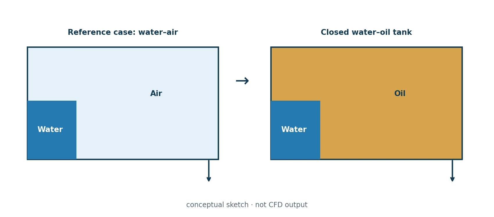
Figure 1 — Conceptual geometry. The actual case is based on the official mesh; the top is open for water–air and closed for water–oil.
Deep dive · The tutorial data sheet, read from its files
| Quantity | Value | File |
|---|---|---|
| tank | 0.584 × 0.584 m, thickness 0.0146 m (one cell) | system/blockMeshDict (scale 0.146) |
| obstacle on the floor | 0.024 m wide, 0.048 m high, between x = 0.292 and 0.316 m | system/blockMeshDict |
| cells | 2268 (5 blocks: 23/4/19 in x, 8 + 42 in y) | system/blockMeshDict |
| cell size | Δx ≈ 12.7 mm (6 mm over the obstacle); Δy = 6 mm below y = 0.048 m, 12.8 mm above | — |
| initial water column | box (0 0 −1) (0.1461 0.292 1), zonal function | 0/alpha.water |
| water | ρ = 1000 kg/m³, ν = 1·10⁻⁶ m²/s | constant/physicalProperties.water |
| air | ρ = 1 kg/m³, ν = 1.48·10⁻⁵ m²/s | constant/physicalProperties.air |
| surface tension | σ = 0.07 N/m | constant/phaseProperties |
| gravity; turbulence | (0 −9.81 0) m/s²; laminar | constant/g, constant/momentumTransport |
| time control | endTime 1; deltaT 0.001; adjustTimeStep yes; maxCo 1; maxAlphaCo 1; maxDeltaT 1; writeInterval 0.05; | system/controlDict |
| α scheme | div(phi,alpha) Gauss interfaceCompression vanLeer 1; | system/fvSchemes |
| MULES controls | "alpha.water.*" { nCorrectors 2; nSubCycles 1; MULESCorr yes; MULES { nIter 10; tolerance 1e-2; } } | system/fvSolution |
| PIMPLE | momentumPredictor no; nOuterCorrectors 1; nCorrectors 3; nNonOrthogonalCorrectors 0; | system/fvSolution |
| top conditions | alpha.water inletOutlet; U pressureInletOutletVelocity; p_rgh prghTotalPressure | 0/* |
Source: tutorials/incompressibleVoF/damBreakLaminar. The system/configDict file activates MULES debug messages (DebugSwitches { MULES 1; }), which is why the log reports the limiter corrections.
Practical tip · How to read a time step in the VoF log
Courant Number mean: 0.0012 max: 0.31
Interface Courant Number mean: 0.0002 max: 0.12
deltaT = 0.00142857
Time = 0.00261905s

PIMPLE: Iteration 1
smoothSolver:  Solving for alpha.water, Initial residual = …, Final residual = …, No Iterations …
Phase-1 volume fraction = 0.130195  Min(alpha.water) = -1e-12  Max(alpha.water) = 1.00000001
MULES: Correcting alpha.water
DICPCG:  Solving for p_rgh, Initial residual = …, Final residual = …, No Iterations …
Courant and deltaT lines precede the Time = line of the step they refer to. “Phase-1 volume fraction” is the volume-weighted mean of αw over the whole domain: multiplied by the domain volume it gives the water inventory at every step, with no post-processing. Min and Max show how well MULES keeps boundedness: deviations of 10⁻⁸–10⁻¹² are normal, values of 10⁻³ or more are not. The example is illustrative; the vof_log_summary.py script (section 8) extracts these lines into a CSV.
2. What physics does VOF represent?
The water–oil exercise considers two immiscible liquids, while the baseline contains a liquid and a gas. In VOF, both fluids are continua and the interface is represented by cell volume fractions, using a single velocity field at the resolved scale. This does not make the substances miscible: intermediate values between alpha.water = 0 and alpha.water = 1 correspond to interface cells.
For two phases, the water volume fraction is αw and the other-phase fraction is α2 = 1 − αw. For constant phase densities, mixture density is ρ = αw ρw + (1−αw)ρ2. Interpreting effective mixture viscosity requires the actual constitutive model; it must not be confused with molecular mixing.
A passive scalar model, as used in Guide 12, does not replace VOF when phase boundaries, gravity and capillary forces matter. Conversely, VOF alone does not solve the distribution of dissolved species between the two immiscible phases.
Deep dive · The equations of the incompressibleVoF module
The incompressibleVoF module solves a single momentum equation for the mixture, with properties weighted by the volume fraction, plus the α transport equation:
rho = alpha*rho_w + (1 - alpha)*rho_2
mu  = a*rho_w*nu_w + (1 - a)*rho_2*nu_2,   a = min(max(alpha, 0), 1)
nu  = mu/(a*rho_w + (1 - a)*rho_2)

d(rho U)/dt + div(rho U U) = - grad(p_rgh) - (g.h) grad(rho) + div(tau) + sigma*kappa*grad(alpha)
kappa = - div( grad(alpha)/|grad(alpha)| )            (CSF, Brackbill et al. 1992)
p_rgh = p - rho (g.h)       (h measured from the reference height)
The mixture properties are computed in incompressibleTwoPhaseVoFMixture.C, with α clipped between 0 and 1 in the viscosity calculation. Surface tension enters as a body force concentrated where ∇α ≠ 0 (CSF model, doi:10.1016/0021-9991(92)90240-Y). The p_rgh formulation moves the hydrostatic term into the density gradient, useful because at rest ∇prgh ≈ 0. The VoF method goes back to Hirt and Nichols, doi:10.1016/0021-9991(81)90145-5; the OpenFOAM implementation (interface compression, MULES) is described by Deshpande, Anumolu, Trujillo, doi:10.1088/1749-4699/5/1/014016.
Deep dive · VoF, Euler–Euler or particles: when to use what
| Situation | Suitable model in OpenFOAM 14 | Criterion |
|---|---|---|
| interface large compared with cells (free surface, separated layers) | incompressibleVoF, compressibleVoF | radius of curvature ≫ Δx |
| many drops or bubbles smaller than cells | multiphaseEuler (interpenetrating phases) | diameter ≲ Δx; a drag and exchange model is needed |
| isolated, dilute particles or drops | Lagrangian clouds (Guide 17) | volume fraction ≲ 10⁻³–10⁻² |
The guide’s water-oil case is a separated-layer problem: VoF is the natural choice. If the motion broke the interface into drops comparable with a cell, VoF would no longer be accurate for those structures.
Practical tip · How to read a cell with intermediate α
A cell with αw = 0.5 does not contain a “mixture” of water and oil: it contains the interface, which the method does not locate inside the cell. In that cell the density used in the momentum equation is 0.5·1000 + 0.5·850 = 925 kg/m³ and the dynamic viscosity is the weighted mean. With interface compression the 0.01 < α < 0.99 zone stays 1–3 cells wide; if it widens over time, the interface is diffusing numerically (scheme, step or mesh).
3. The interface transport equation
The ideal transport equation for a phase fraction is ∂αw/∂t + ∇·(αw U) = 0, for an incompressible flow without interphase mass transfer. Numerically, interface compression is used to limit artificial spreading of the resolved interface, while MULES applies boundedness control to maintain 0 ≤ αw ≤ 1 within numerical tolerances.
The αw = 0.5 contour is a useful interface visualisation convention, not a material wall or a unique physical thickness. The field p_rgh removes a hydrostatic contribution from pressure; it should not be read as the total pressure in pascals. In gravity-driven flow, the practical definition is p_rgh = p − ρ(g·x), with the solver’s adopted height reference.
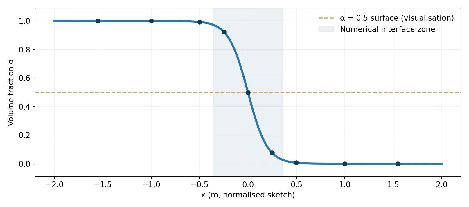
Figure 2 — A schematic volume-fraction profile, not an OpenFOAM solution. The 0.5 contour identifies the visualisation interface.
Optional refresher — dimensionless groups. The Reynolds number compares inertia to viscous effects (Re = ρUL/μ), the Weber number compares inertia to capillary forces (We = ρU²L/σ) and the Bond number compares buoyancy/gravity to capillarity (Bo = ΔρgL²/σ). In gravity separation, density contrast, geometry and time scale are important. The value σ = 0.030 N/m below is an illustrative teaching value, not a universal value for every water–oil system.
Deep dive · Interface compression and MULES in detail
The interfaceCompression vanLeer 1 scheme computes the α flux with the van Leer limiter and adds a compression flux proportional to cα|U|·n α(1 − α) (here cα = 1), acting only where 0 < α < 1 and normal to the interface: it is equivalent to the ∇·(Ur α(1 − α)) term of the modified equation. MULES (Multidimensional Universal Limiter for Explicit Solution) is a flux-corrected-transport limiter (Zalesak, doi:10.1016/0021-9991(79)90051-2) that corrects the fluxes so that α stays between 0 and 1.
MULESCorr yes: first an implicit upwind solution, then the limited higher-order correction; allows higher interface Courant numbers.nCorrectors 2: two α correction loops per step;nSubCycles 1: no sub-cycling. IndamBreak3DandcapillaryRiseversion 14 usesnSubCycles polynomial (0 4), i.e. a number of sub-cycles that is a function of the Courant number.- Geometric alternatives:
Gauss PLICandGauss MPLICreconstruct the interface by planes within the cell; the damBreak3D tutorial usesdiv(phi,alpha) Gauss MPLIC;.
Deep dive · Dimensionless numbers of the four runs (vof_estimates.py script)
| Case | Δρ | g′ (m/s²) | U = √(g′H) | Re2 | Bo(H) | ℓc = √(σ/Δρg) | cells per ℓc |
|---|---|---|---|---|---|---|---|
| water_air_reference | 999 | 9.80 | 1.69 m/s | 33 400 | 11 900 | 2.67 mm | 0.21 |
| water_oil_reference | 150 | 1.59 | 0.68 m/s | 3 980 | 4 180 | 4.52 mm | 0.36 |
| water_oil_low_sigma | 150 | 1.59 | 0.68 m/s | 3 980 | 12 500 | 2.61 mm | 0.21 |
| water_oil_high_nu | 150 | 1.59 | 0.68 m/s | 1 990 | 4 180 | 4.52 mm | 0.36 |
H = 0.292 m is the column height; for the water-oil cases the reduced gravity is g′ = gΔρ/ρ̄ with ρ̄ = 925 kg/m³. Important consequence: the capillary length (2.6–4.5 mm) is smaller than one cell (12.7 mm). Even at the scale of one cell the Bond number Δρ g Δx²/σ is about 8 (oil, σ = 0.03), 24 (oil, σ = 0.01) and 23 (air): gravity dominates resolved surface tension everywhere. It is therefore predictable that the water_oil_reference / water_oil_low_sigma comparison will show small differences in the large-scale dynamics, comparable with the numerical error; observing capillary effects would require a mesh at least 5–10 times finer near the interface. The water-side Reynolds number U H/νw is of the order of 10⁵: the laminar model is a modelling choice, not a consequence of the physics.
#!/usr/bin/env python3
# SPDX-License-Identifier: GPL-3.0-or-later
"""Scale analysis for the Guide 13 VOF cases (damBreakLaminar geometry).

Mesh from the official blockMeshDict (scale 0.146): domain 0.584 x 0.584 m,
one cell (0.0146 m) thick, 2268 cells of about 12.7 mm; water column
0.1461 x 0.292 m. Properties from the guide's table. Prints density contrast,
reduced gravity, velocity and time scales, Reynolds, Bond and Weber numbers,
capillary length versus cell size, and the explicit capillary time-step limit.
Order-of-magnitude checks only, not CFD results.
"""
import argparse
import math

CASES = {
    'water_air_reference': (1.0, 1.48e-5, 0.070),
    'water_oil_reference': (850.0, 5e-5, 0.030),
    'water_oil_low_sigma': (850.0, 5e-5, 0.010),
    'water_oil_high_nu': (850.0, 1e-4, 0.030),
}


def main():
    p = argparse.ArgumentParser(description=__doc__)
    p.add_argument('--dx', type=float, default=0.584 / 46, help='cell size [m]')
    p.add_argument('--H', type=float, default=0.292, help='water column height [m]')
    p.add_argument('--W', type=float, default=0.1461, help='water column width [m]')
    p.add_argument('--g', type=float, default=9.81)
    a = p.parse_args()
    rho_w, nu_w = 1000.0, 1e-6
    print(f'cell size {a.dx * 1000:.1f} mm; water area {a.W * a.H:.4e} m2, volume (1 cell thick) {a.W * a.H * 0.0146:.4e} m3')
    print('case                  drho   g_red  U=sqrt(g_red H)  t=H/U   Re_2nd  Bo(H)    We     l_cap  cells/l_cap  dt_cap')
    for name, (rho2, nu2, sigma) in CASES.items():
        drho = rho_w - rho2
        rho_m = 0.5 * (rho_w + rho2)
        g_red = a.g * drho / rho_w if rho2 < 10 else a.g * drho / rho_m
        U = math.sqrt(g_red * a.H)
        t = a.H / U
        re2 = U * a.H / nu2
        bo = drho * a.g * a.H ** 2 / sigma
        we = rho_m * U ** 2 * a.H / sigma
        lcap = math.sqrt(sigma / (drho * a.g))
        dt_cap = math.sqrt(rho_m * a.dx ** 3 / (2 * math.pi * sigma))
        print(f'{name:21s} {drho:5.0f}  {g_red:5.2f}   {U:8.3f}       {t:6.3f}  {re2:7.0f}  {bo:7.0f}  {we:6.0f}  {lcap * 1000:5.2f} mm  {lcap / a.dx:6.2f}     {dt_cap:.3g} s')
    print('Water side Reynolds number U H / nu_w is about 1e5 for every case: the laminar model is a modelling choice.')


if __name__ == '__main__':
    main()
Deep dive · Capillary time-step limit and parasitic currents
With explicit surface tension the step must also satisfy Δt < √(ρ̄ Δx³/(2πσ)) (Brackbill et al. 1992; analysis revisited by Denner and van Wachem, doi:10.1016/j.jcp.2015.01.021). With Δx = 12.7 mm the limit is about 0.05 s for water-air and 0.1–0.17 s for water-oil, much looser than the Courant limit (Δx/U ≈ 8–19 ms): it is not binding here, but becomes dominant when the mesh is refined, because it scales with Δx3/2 instead of Δx.
“Parasitic currents” are spurious velocities generated by the curvature error near interfaces at rest; Popinet’s review, doi:10.1146/annurev-fluid-122316-045034, describes causes and remedies. A simple check: in the final stratified state the maximum velocity (UmaxMag in the functions file) must decay towards zero; a non-zero plateau indicates parasitic currents or an undamped oscillation.
4. Official case and version-specific syntax
The authoritative starting point is the OpenFOAM Foundation 14 tutorial incompressibleVoF/damBreakLaminar. It specifies solver incompressibleVoF; in system/controlDict and uses foamRun for execution. Avoid copying historical dictionaries for interFoam, transportProperties or turbulenceProperties from a different OpenFOAM edition.
The base case contains 0/alpha.water, 0/U, 0/p_rgh, constant/phaseProperties, constant/physicalProperties.water, constant/physicalProperties.air, constant/g, constant/momentumTransport and the usual system/ dictionaries. OpenFOAM 14 allows nonuniform initialisation of alpha.water through a zonal function in the internalField entry; a separate compulsory setFields preprocessing stage is not required for this case.
Verified references: Foundation 14 user guide: https://doc.cfd.direct/openfoam/user-guide-v14/dambreak ; official sources: https://github.com/OpenFOAM/OpenFOAM-14/tree/master/tutorials/incompressibleVoF/damBreakLaminar .
Deep dive · The zonal initialisation snaps to cell centres
The zonal function assigns α = 1 to cells whose centre lies in the box. With Δx = 12.70 mm and Δy = 6 mm / 12.76 mm the actual column is 12 cells × 0.012696 m = 0.15235 m wide and (8 × 0.006 + 19 × 0.012762) = 0.29048 m high: an area of 0.044253 m², 3.7 % more than the nominal box 0.1461 × 0.292 = 0.042661 m². The initial phase fraction printed in the log is therefore about 0.1302 (domain area 0.339904 m²). For relative conservation errors use the first log value or the first volIntegrate(alpha.water) as the reference, never the nominal box volume.
Function documentation: Foundation 14 user guide, field functions. The command foamDictionary 0/alpha.water -entry internalField shows the definition without opening an editor.
Deep dive · Other version 14 VoF tutorials useful for this guide
| Tutorial | What it shows |
|---|---|
| damBreakTracer | phaseScalarTransport of a tracer in water and in air (bridge to Guide 12 and section 16) |
| damBreak3D | three-dimensional version with the MPLIC scheme |
| sloshingTank2D | closed tank with pRefPoint and pRefValue (section 5) |
| capillaryRise | surface-tension-dominated case, with contact angle |
| mixerVessel2DMRF, testTubeMixer | mixers and moving vessels (Guides 15–16) |
5. The four independent experiments
The accompanying scripts never modify the installed OpenFOAM tutorial. prepare_cases.py copies the original into four new folders and refuses to proceed if the destination already exists:
Guide13_cases/
  water_air_reference/
  water_oil_reference/
  water_oil_low_sigma/
  water_oil_high_nu/
The water–air baseline keeps its open atmosphere boundary. In all three water–oil variants, this boundary is turned into a closed upperWall; the air phase becomes oil, illustrative oil properties are set, and the boundary conditions of alpha.water, U and p_rgh are adjusted. The reference mesh and initial water column remain unchanged to support controlled comparisons.
Deep dive · WARNING: the three closed water-oil cases do not start without a pressure reference
In the water-oil cases the script turns the top boundary into a wall with p_rgh of type fixedFluxPressure. All boundaries then impose the flux and the pressure level is undetermined: OpenFOAM 14 requires a reference in the PIMPLE dictionary of system/fvSolution and, if it is missing, stops immediately with the error from findRefCell.C:
--> FOAM FATAL IO ERROR:
Unable to set reference cell for field p
    Please supply either pRefCell or pRefPoint
The official closed-tank tutorials do this: sloshingTank2D declares pRefPoint (0 0 0.15); pRefValue 1e5;. The following additional script inserts pRefPoint (0.292 0.55 0.0073); pRefValue 0; (a point in the oil, below the lid and at mid-thickness) into the three prepared, not yet run water-oil cases, keeping system/fvSolution.noPressureReference. It was tested on real copies prepared from the OpenFOAM 14 tutorial. The value 0 is legitimate in an incompressible flow: only the pressure gradient matters.
python3 prepare_cases.py --destination "$HOME/cases/Guide13_cases"
python3 add_pressure_reference.py "$HOME/cases/Guide13_cases"
foamDictionary "$HOME/cases/Guide13_cases/water_oil_reference/system/fvSolution" -entry PIMPLE
#!/usr/bin/env python3
# SPDX-License-Identifier: GPL-3.0-or-later
"""Add a pressure reference to the closed water-oil cases of Guide 13.
In a closed domain every p_rgh boundary is fixedFluxPressure, so the pressure
level is undetermined. OpenFOAM 14 (pressureReference -> setRefCell) then
requires pRefCell or pRefPoint plus pRefValue in the PIMPLE dictionary of
system/fvSolution, otherwise the run stops with
"Unable to set reference cell for field p". The official closed-tank VoF
tutorials (sloshingTank2D, sloshingCylinder, ...) set these entries.
Only prepared, not yet run copies are modified; the original fvSolution is kept
as system/fvSolution.noPressureReference.
"""
import argparse
from pathlib import Path
import re
import sys
OIL_CASES = ('water_oil_reference', 'water_oil_low_sigma', 'water_oil_high_nu')
def main():
p = argparse.ArgumentParser(description=__doc__)
p.add_argument('cases_root', type=Path, help='folder created by prepare_cases.py')
p.add_argument('--point', default='(0.292 0.55 0.0073)',
help='reference point inside the fluid domain [m] (default: top centre)')
p.add_argument('--value', default='0', help='pRefValue [Pa]')
a = p.parse_args()
root = a.cases_root.expanduser().resolve()
for name in OIL_CASES:
case = root / name
f = case / 'system' / 'fvSolution'
if not (case / 'GUIDE13_CASE.txt').is_file() or not f.is_file():
p.error(f'{case} is not a prepared Guide 13 case')
if (case / 'log.foamRun').exists():
p.error(f'{name} has already been run; prepare a fresh case instead')
text = f.read_text(encoding='utf-8')
if re.search(r'\bpRef(Cell|Point)\b', text):
print(f'{name}: pressure reference already present, unchanged')
continue
m = re.search(r'(?m)^PIMPLE\s*\{', text)
if not m:
p.error(f'{f}: PIMPLE dictionary not found')
backup = f.with_name('fvSolution.noPressureReference')
if backup.exists():
p.error(f'{backup} exists; refusing to overwrite it')
backup.write_text(text, encoding='utf-8')
insert = f'\n pRefPoint {a.point};\n pRefValue {a.value};\n'
f.write_text(text[:m.end()] + insert + text[m.end():], encoding='utf-8')
print(f'{name}: pRefPoint {a.point}, pRefValue {a.value} added to PIMPLE')
if __name__ == '__main__':
try:
main()
except OSError as exc:
sys.exit(f'ERROR: {exc}')Deep dive · Package script: prepare_cases.py
It checks that the source is a version 14 incompressibleVoF case without mesh or results, builds the four copies in a temporary folder next to the destination and renames it only at the end (atomic operation). For the water-oil cases: it replaces phases (water air) with (water oil) and the sigma value; renames physicalProperties.air to physicalProperties.oil with ρ = 850 and the new ν; turns atmosphere into upperWall (type wall) in blockMeshDict and in the 0/ fields. Every substitution must happen exactly once, otherwise the procedure stops.
#!/usr/bin/env python3
# SPDX-License-Identifier: GPL-3.0-or-later
"""Prepare safe, independent OpenFOAM Foundation 14 VOF tutorial variants."""
import argparse
import os
from pathlib import Path
import re
import shutil
import sys
import tempfile

VARIANTS = {
    'water_air_reference': (False, 0.07, 1.48e-5),
    'water_oil_reference': (True, 0.030, 5e-5),
    'water_oil_low_sigma': (True, 0.010, 5e-5),
    'water_oil_high_nu': (True, 0.030, 1e-4),
}


def replace_exact(s, old, new, file):
    n = s.count(old)
    if n != 1:
        raise ValueError(f'{file}: expected one occurrence of {old!r}, found {n}')
    return s.replace(old, new)


def substitute_entry(s, key, val, file):
    pat = re.compile(r'(?m)^([ \t]*' + re.escape(key) + r'[ \t]+)([^;\n]+)(;)')
    hits = len(pat.findall(s))
    if hits != 1:
        raise ValueError(f'{file}: expected one entry {key}, found {hits}')
    return pat.sub(lambda m: m.group(1)+str(val)+m.group(3),s,count=1)


def replace_patch(s, patch, content, file):
    pat = re.compile(r'(?ms)^([ \t]*)'+re.escape(patch)+r'[ \t]*\n[ \t]*\{[^{}]*?^[ \t]*\}',re.M)
    found = list(pat.finditer(s))
    if len(found) != 1:
        raise ValueError(f'{file}: patch {patch} match count {len(found)}')
    indent = found[0].group(1)
    body = '\n'.join(indent+'    '+x for x in content)
    return s[:found[0].start()]+f'{indent}{patch}\n{indent}{{\n{body}\n{indent}}}'+s[found[0].end():]


def patch_file(root, rel, change):
    p=root/rel
    old=p.read_text(encoding='utf-8')
    new=change(old,rel)
    p.write_text(new, encoding='utf-8', newline='\n')


def to_oil(root,sigma,nu):
    rel='constant/phaseProperties'
    def phases(s,f):
        s=replace_exact(s,'phases          (water air);','phases          (water oil);',f)
        return substitute_entry(s,'sigma',f'{sigma:.3f}',f)
    patch_file(root,rel,phases)
    orig=root/'constant/physicalProperties.air'
    renamed=root/'constant/physicalProperties.oil'
    if renamed.exists():raise ValueError('Oil property file already exists')
    orig.rename(renamed)
    def prop(s,f):
        s=replace_exact(s,'object      physicalProperties.air;','object      physicalProperties.oil;',f)
        s=substitute_entry(s,'nu',f'{nu:.8g}',f)
        return substitute_entry(s,'rho','850',f)
    patch_file(root,'constant/physicalProperties.oil',prop)
    for rel,content in [
        ('0/alpha.water',['type            zeroGradient;']),
        ('0/U',['type            noSlip;']),
        ('0/p_rgh',['type            fixedFluxPressure;','value           $internalField;']),
    ]:
        def change(s,f):
            s=replace_exact(s,'atmosphere','upperWall',f)
            return replace_patch(s,'upperWall',content,f)
        patch_file(root,rel,change)
    def topmesh(s,f):
        s=replace_exact(s,'atmosphere','upperWall',f)
        def patch_block(m):
            block=m.group(0)
            if block.count('type patch;')!=1:
                raise ValueError('top patch does not have exactly one type patch')
            return block.replace('type patch;','type wall;')
        pat=re.compile(r'(?ms)^[ \t]*upperWall\s*\{[^{}]*?^[ \t]*\}',re.M)
        if len(pat.findall(s))!=1:raise ValueError('upperWall block not unique')
        return pat.sub(patch_block,s,count=1)
    patch_file(root,'system/blockMeshDict',topmesh)
    return root


def validate_source(source):
    required=['0/alpha.water','0/U','0/p_rgh','constant/phaseProperties',
              'constant/physicalProperties.air','constant/physicalProperties.water',
              'system/blockMeshDict','system/controlDict','system/fvSolution']
    missing=[p for p in required if not (source/p).is_file()]
    if missing: raise ValueError(f'Missing official tutorial files: {missing}')
    if (source/'constant/polyMesh').exists() or any(source.glob('processor[0-9]*')):
        raise ValueError('Refusing source with generated mesh or decomposed results')
    ctrl=(source/'system/controlDict').read_text()
    if 'solver          incompressibleVoF;' not in ctrl:
        raise ValueError('Not an OpenFOAM Foundation v14 incompressibleVoF case')


def main():
    a=argparse.ArgumentParser(description=__doc__)
    a.add_argument('--destination',type=Path,required=True,help='NEW output folder, must not exist')
    a.add_argument('--source',type=Path,help='Official damBreakLaminar case path')
    args=a.parse_args()
    source=args.source
    if source is None:
        tutorials=os.environ.get('FOAM_TUTORIALS')
        if not tutorials:
            a.error('FOAM_TUTORIALS unset: source OpenFOAM first or use --source')
        source=Path(tutorials)/'incompressibleVoF/damBreakLaminar'
    source=source.resolve()
    validate_source(source)
    target=args.destination.expanduser().resolve()
    if target.exists():raise ValueError(f'Destination already exists: {target}')
    if not target.parent.is_dir():raise ValueError(f'Parent directory missing: {target.parent}')
    if target == source or source in target.parents:
        raise ValueError('Destination may not be located inside the official source tutorial')
    stage=Path(tempfile.mkdtemp(prefix='.guide13_build_',dir=target.parent))
    try:
        for name,(oil,sigma,nu) in VARIANTS.items():
            dest=stage/name
            shutil.copytree(source,dest)
            if oil:to_oil(dest,sigma,nu)
            (dest/'GUIDE13_CASE.txt').write_text(
                f'Guide 13 case: {name}\nBased on OpenFOAM Foundation 14 tutorial '
                'incompressibleVoF/damBreakLaminar.\n'
                'No simulation has been performed yet.\n'
                f'Closed oil-water tank: {oil}\nSurface tension: {sigma} N/m\n'
                f'Second-phase kinematic viscosity: {nu} m2/s\n',encoding='utf-8')
        stage.rename(target)
    except BaseException:
        shutil.rmtree(stage,ignore_errors=True)
        raise
    print(f'Created {len(VARIANTS)} independent, uncomputed cases at: {target}')
    for name in VARIANTS:print('  -',name)
    print('No original tutorial files were modified.')


if __name__=='__main__':
    try:main()
    except (ValueError,OSError) as e:
        print('ERROR:',e,file=sys.stderr)
        sys.exit(2)
Deep dive · Water-oil properties: orders of magnitude
ρ = 850 kg/m³ and ν = 5·10⁻⁵ m²/s (μ ≈ 0.043 Pa·s) are typical of a light mineral oil; ν = 10⁻⁴ m²/s doubles the viscosity. The interfacial tension between pure water and saturated hydrocarbons is of the order of 0.05 N/m; impurities and surfactants reduce it even by orders of magnitude, so 0.03 and 0.01 N/m are plausible choices but must be replaced by measurements (pendant-drop or ring tensiometer) for any experimental comparison. The oil/water dynamic viscosity ratio is about 43 (85 in the high_nu case): oscillation damping occurs mainly in the oil.
Physical parameters
| Folder | Phases | Top boundary | σ (N/m) | Second-phase ν (m²/s) |
|---|---|---|---|---|
water_air_reference | water/air | open | 0.070 | 1.48×10⁻⁵ |
water_oil_reference | water/oil | closed | 0.030 | 5.0×10⁻⁵ |
water_oil_low_sigma | water/oil | closed | 0.010 | 5.0×10⁻⁵ |
water_oil_high_nu | water/oil | closed | 0.030 | 1.0×10⁻⁴ |
The water–oil exercises retain the official ρwater = 1000 kg/m³ and use an illustrative ρoil = 850 kg/m³. Replace these values with measured or reliable fluid properties before making experimental claims.
6. Prepare the cases from the Linux server
Upload the included scripts/ folder to a working directory via FileZilla/SFTP. From Windows PowerShell, connect by ssh user@server-host. On the remote server, source Foundation 14 if it is not already loaded:
source /opt/OpenFOAM-14/etc/bashrc
foamVersion
python3 prepare_cases.py --destination "$HOME/cases/Guide13_cases"
Change the source path if the installation resides elsewhere. The script relies on FOAM_TUTORIALS or accepts --source /path/to/damBreakLaminar. Python 3 is required. The destination path must not exist, but its parent directory must exist. Do not use sudo.
Before running, inspect constant/phaseProperties in the water–oil variants: it must contain phases (water oil);. Check physicalProperties.oil, the upperWall patch and system/controlDict.
Practical tip · Checking the prepared cases before launch
cd "$HOME/cases/Guide13_cases"
for c in water_air_reference water_oil_reference water_oil_low_sigma water_oil_high_nu; do
  echo "== $c"
  foamDictionary $c/constant/phaseProperties -entry phases
  foamDictionary $c/constant/phaseProperties -entry sigma
  ls $c/constant/physicalProperties.*
  grep -A3 "upperWall\|atmosphere" $c/system/blockMeshDict | head -n 4
  foamDictionary $c/system/fvSolution -entry PIMPLE | grep -E "pRef" || echo "  no pressure reference"
done
Expected outcome: the water-air case with (water air), σ = 0.07, atmosphere boundary and no reference (not needed, the boundary is open); the three water-oil cases with (water oil), correct σ, physicalProperties.oil, upperWall of type wall and the added pressure reference.
Practical tip · Transfer from Windows: line endings
file scripts/*.sh scripts/*.py              # "CRLF line terminators" means Windows endings
sed -i 's/\r$//' scripts/run_case.sh       # only if needed
bash -n scripts/run_case.sh                   # syntax check without running
Use binary transfer mode in FileZilla for scripts; Python 3.8 or later is enough (standard library only).
7. Run the simulations sequentially
The following command runs blockMesh, checkMesh and foamRun, retaining separate log files:
bash run_case.sh "$HOME/cases/Guide13_cases/water_air_reference"Run the other cases by changing only the folder name. For long jobs, use tmux new -s vof13, start the job, detach with Ctrl+B then D, and reconnect with tmux attach -t vof13. Avoid launching all four runs in parallel without checking memory, CPU quotas and other server users.
run_case.sh refuses to overwrite existing logs, meshes or completion markers. If a case fails, examine the logs and prepare a fresh run directory rather than deleting evidence. Outputs include log.blockMesh, log.checkMesh, log.foamRun, and .guide13_completed only after the program exits successfully.
Verification warning. The completion marker confirms successful process exit only. It does not prove mass conservation, grid independence or physical validation.
Deep dive · Package script: run_case.sh
It checks that the folder is a guide case and that the OpenFOAM environment is active, refuses existing logs, meshes and markers, then runs blockMesh, checkMesh and foamRun with set -euo pipefail. If foamRun fails (for example because of the missing pressure reference) the script exits with an error, the log remains and the .guide13_completed marker is not created; a new attempt requires a fresh copy, because the existing log blocks repetition.
#!/usr/bin/env bash
# SPDX-License-Identifier: GPL-3.0-or-later
# Run one fresh Guide 13 case without deleting or overwriting existing results.
set -euo pipefail
if (( $# != 1 )); then
  echo "Usage: bash run_case.sh /path/to/one/guide13/case" >&2
  exit 2
fi
case_dir=$(realpath -- "$1")
[[ -f "$case_dir/system/controlDict" && -f "$case_dir/GUIDE13_CASE.txt" ]] || { echo "Not a Guide 13 case" >&2; exit 2; }
command -v blockMesh >/dev/null || { echo "OpenFOAM environment not sourced" >&2; exit 2; }
command -v foamRun >/dev/null || { echo "foamRun not available" >&2; exit 2; }
for f in log.blockMesh log.checkMesh log.foamRun .guide13_completed; do
  [[ ! -e "$case_dir/$f" ]] || { echo "Refusing overwrite: $case_dir/$f" >&2; exit 3; }
done
[[ ! -d "$case_dir/constant/polyMesh" ]] || { echo "Mesh already exists; create a fresh case" >&2; exit 3; }
cd -- "$case_dir"
echo "Running blockMesh in $case_dir"
blockMesh > log.blockMesh 2>&1
checkMesh > log.checkMesh 2>&1
echo "Running foamRun; logs retained even if the run fails"
foamRun > log.foamRun 2>&1
touch .guide13_completed
echo "Case complete: $case_dir (inspect log.foamRun and physical diagnostics)"
Deep dive · Measuring during the run: a system/functions file for VoF
The tutorial has no system/functions file. The following file (with the FoamFile header, essential for OpenFOAM 14 to read it) must be copied into the system folder of each case before run_case.sh. At every step it records the water inventory ∫α dV, the interface height above four stations on the floor (left wall, middle of the left chamber, behind the obstacle, right wall) and the maximum velocity. The interfaceHeight function object uses an integral method: with several interfaces on the same vertical it returns averaged values.
/*--------------------------------*- C++ -*----------------------------------*\
  Guide 13 - monitoring functions for a NEW damBreakLaminar copy.
  Save as <case>/system/functions BEFORE run_case.sh.
\*---------------------------------------------------------------------------*/
FoamFile
{
    format      ascii;
    class       dictionary;
    location    "system";
    object      functions;
}

// Water inventory integral(alpha.water dV) [m3] at every time step
#includeFunc volIntegrate(alpha.water)

// Height of the water above four stations on the floor [m] (integral method):
// left wall (residual column), mid-tank, behind the obstacle, right wall
interfaceHeight1
{
    type            interfaceHeight;
    libs            ("libfieldFunctionObjects.so");
    alpha           alpha.water;
    locations       ((0.0073 0.001 0.0073) (0.146 0.001 0.0073) (0.45 0.001 0.0073) (0.577 0.001 0.0073));
}

// Largest velocity magnitude in the domain [m/s]
#includeFunc cellMaxMag(name=UmaxMag, U)

// ************************************************************************* //
for c in water_air_reference water_oil_reference water_oil_low_sigma water_oil_high_nu; do
cp -n functions_guide13 "$HOME/cases/Guide13_cases/$c/system/functions"
done
ls "$HOME/cases/Guide13_cases/water_oil_reference/postProcessing" # after the runPractical tip · Run duration and sequence
With 2268 cells each case usually takes from a few seconds to a few minutes on one core. The four cases can be run one after the other in a tmux session:
cd "$HOME/cases/Guide13_cases"
for c in water_air_reference water_oil_reference water_oil_low_sigma water_oil_high_nu; do
  bash ~/scripts/run_case.sh "$PWD/$c" || { echo "stopped at $c"; break; }
done
8. Time-step control, MULES and stability
The official controlDict uses adjustTimeStep yes, maxCo 1, maxAlphaCo 1 and writeControl adjustableRunTime. These are tutorial defaults, not universal accuracy guarantees. A smaller step may be needed for high surface tension, thin cells or fast capillary dynamics.
In fvSchemes, phase advection uses div(phi,alpha) Gauss interfaceCompression vanLeer 1;. In fvSolution, the "alpha.water.*" group sets MULES controls and phase corrections. When studying the effect of a physical parameter, avoid changing multiple numerical settings simultaneously. Report the maximum Courant number, warnings, actual steps and cell count for every run.
Deep dive · Additional script: vof_log_summary.py
It extracts from log.foamRun, for every step, maximum Courant, interface Courant, deltaT, phase fraction, relative inventory drift and α bounds, correctly assigning the Courant lines to the following step. It writes a new CSV and a summary. Tested on a log excerpt with the OpenFOAM 14 structure.
python3 vof_log_summary.py water_oil_reference/log.foamRun --output vof_summary_oil_ref.csv#!/usr/bin/env python3
# SPDX-License-Identifier: GPL-3.0-or-later
"""Summarise an OpenFOAM 14 incompressibleVoF log (log.foamRun).
For every time step the VoF solver prints, among others:
Courant Number mean: ... max: ...
Interface Courant Number mean: ... max: ...
deltaT = ...
Time = ...
Phase-1 volume fraction = ... Min(alpha.water) = ... Max(alpha.water) = ...
Courant numbers and deltaT precede the 'Time =' line of their step and are
assigned to that step. The phase-1 volume fraction is the volume-weighted mean of alpha.water over
the domain, so (fraction - fraction_0)/fraction_0 is the relative drift of the
water inventory, available without any post-processing. Writes a NEW CSV with
one row per time step (last printed values) and prints a short summary.
"""
import argparse
import csv
from pathlib import Path
import re
import sys
NUM = r'([-+0-9.eE]+)'
PATTERNS = {
'Co_max': re.compile(r'^Courant Number mean: ' + NUM + r' max: ' + NUM),
'alphaCo_max': re.compile(r'^Interface Courant Number mean: ' + NUM + r' max: ' + NUM),
'deltaT': re.compile(r'^deltaT = ' + NUM),
'phase': re.compile(r'^Phase-1 volume fraction = ' + NUM + r'\s+Min\((\S+)\) = ' + NUM + r'\s+Max\(\S+\) = ' + NUM),
}
def main():
p = argparse.ArgumentParser(description=__doc__, formatter_class=argparse.RawDescriptionHelpFormatter)
p.add_argument('log', type=Path)
p.add_argument('--output', type=Path, required=True, help='NEW csv file')
a = p.parse_args()
if a.output.exists():
p.error('Output exists; refusing to overwrite it')
rows, cur, pending = [], None, {}
with a.log.open(encoding='utf-8', errors='replace') as f:
for line in f:
s = line.strip()
m = re.match(r'^Time = ' + NUM + r's?$', s)
if m:
if cur and 'fraction' in cur:
rows.append(cur)
# Courant numbers and deltaT are printed just before 'Time =' of their step
cur = {'time': float(m.group(1))}
cur.update(pending)
pending = {}
continue
for key, pat in PATTERNS.items():
m = pat.match(s)
if not m:
continue
if key == 'phase':
if cur is None:
break
cur['fraction'] = float(m.group(1))
cur['alpha_min'] = float(m.group(3))
cur['alpha_max'] = float(m.group(4))
elif key == 'deltaT':
pending['deltaT'] = float(m.group(1))
else:
pending[key] = float(m.group(2))
if cur and 'fraction' in cur:
rows.append(cur)
if not rows:
p.error('No "Phase-1 volume fraction" lines found: is this an incompressibleVoF log?')
f0 = rows[0]['fraction']
with a.output.open('x', newline='', encoding='utf-8') as f:
w = csv.writer(f)
w.writerow(['time_s', 'deltaT_s', 'Co_max', 'interface_Co_max', 'phase1_fraction', 'relative_drift', 'alpha_min', 'alpha_max'])
for r in rows:
w.writerow([r['time'], r.get('deltaT', ''), r.get('Co_max', ''), r.get('alphaCo_max', ''),
f"{r['fraction']:.10g}", f"{(r['fraction'] - f0) / f0:.4e}" if f0 else 'nan',
r['alpha_min'], r['alpha_max']])
last = rows[-1]
print(f'{len(rows)} time steps, t = {rows[0]["time"]:g} ... {last["time"]:g} s')
print(f'phase-1 fraction: first {f0:.8g}, last {last["fraction"]:.8g}, relative drift {(last["fraction"] - f0) / f0:.3e}')
print(f'max Courant {max(r.get("Co_max", 0) for r in rows):.3g}, max interface Courant {max(r.get("alphaCo_max", 0) for r in rows):.3g}')
print(f'alpha range over the run: [{min(r["alpha_min"] for r in rows):.3g}, {max(r["alpha_max"] for r in rows):.6g}]')
dts = [r['deltaT'] for r in rows if 'deltaT' in r]
if dts:
print(f'deltaT range: {min(dts):.3g} ... {max(dts):.3g} s')
print('Written', a.output)
if __name__ == '__main__':
try:
main()
except OSError as exc:
sys.exit(f'ERROR: {exc}')Deep dive · Numerical sensitivity plan, one change at a time
| Test | Change (in a new copy) | What it measures |
|---|---|---|
| step | maxCo 0.5; maxAlphaCo 0.5; | time error |
| sub-cycles | nSubCycles 3; in the alpha.water dictionary | accuracy of α transport |
| scheme | div(phi,alpha) Gauss MPLIC; | numerical interface diffusion |
| mesh | cells doubled in every block: (46 16 1), (38 16 1), (46 84 1), (8 84 1), (38 84 1) | spatial error (Guide 4) |
Unlike Guide 12, here the mesh can be refined freely because it is generated by blockMesh and the initial fields are defined by functions, not by value lists. With a doubled mesh the cell count rises to 9072 and the step halves: the cost grows by about 8 times in 2D.
Deep dive · Courant and interface Courant: what limits the step
The cell Courant number is Co = ½ Σ|φf| Δt / V; the interface Courant is the same quantity evaluated only in the cells containing the interface (0 < α < 1). With adjustTimeStep yes the next step is chosen so that both stay below maxCo and maxAlphaCo and below maxDeltaT; increases are gradual to avoid oscillations. In the log, therefore, the maximum Courant hovers around 1 in the fast phases: this is not an error, it is the control at work. The actual step (deltaT = line) is the quantity to report.
9. Gravity, volume and pressure
In the official tutorial, gravity is g = (0 −9.81 0) m/s², so y is the vertical coordinate. The mesh is a single cell thick in z, with empty front/back boundaries: it is a numerically two-dimensional case, not a resolved three-dimensional experimental tank. Integrated volumes include the extruded geometrical thickness and should not be interpreted as volumes from a 3D vessel without explicit scaling.
The water–oil evolution reflects density contrast, initial water distribution, viscosity and surface tension. There is no guarantee of perfect separation within one simulated second; numerical interface diffusion or spurious currents may influence the outcome.
Deep dive · What to expect: time scales and final state
- Water-air. The front advances at a speed of the order of √(gH) ≈ 1.7 m/s (up to 2√(gH) ≈ 3.4 m/s in Ritter’s shallow-water solution) and reaches the obstacle, 0.14 m beyond the column, in less than 0.1 s; it then hits the right wall and falls back. The sequence is the classical Martin and Moyce problem, doi:10.1098/rsta.1952.0006.
- Water-oil. The motion is a gravity current with a small density difference: the front speed is of the order of 0.5√(g′H), i.e. 0.35–0.5 m/s depending on whether H is taken as the column height (0.292 m) or the tank height (0.584 m) (theory of Benjamin, J. Fluid Mech. 1968), so crossing the tank takes 1–2 s and the following oscillations last much longer. With
endTime 1the oil case is still far from equilibrium: to study separation setendTimeto 10–20 s in a new copy (the cost stays modest).
The final stratified state follows from the geometry: the vof_equilibrium.py script (next box) predicts a water level of 0.0778 m, a water centroid falling from 0.1452 to 0.0393 m and a released potential energy of about 6.9 J per metre of depth in the water-oil case. These are the asymptotic values against which to compare interfaceHeight and the centroids computed by phase_metrics.py.
Deep dive · Additional script: vof_equilibrium.py
It rebuilds the blockMeshDict mesh (cell centres and sizes), applies the cell-centre criterion of the zonal function and computes the actual inventory, the phase fraction expected in the log, the final level, the initial and final centroids of the two phases and the released potential energy. With --rho2 1 it gives the values for the water-air case (where, however, the final state is never reached within 1 s).
#!/usr/bin/env python3
# SPDX-License-Identifier: GPL-3.0-or-later
"""Initial inventory and stratified end state of the damBreakLaminar geometry.

Geometry from the OpenFOAM 14 blockMeshDict (scale 0.146): tank 0.584 x 0.584 m,
one cell (0.0146 m) thick, obstacle 0.024 m wide and 0.048 m high at
x = 0.292 m, mesh 23+4+19 cells in x and 8+42 cells in y. The zonal initial
condition sets alpha = 1 in cells whose CENTRE lies in the box
(0 0 -1) (0.1461 0.292 1): the real water column is therefore snapped to the
mesh. The script prints the nominal and the snapped inventory, the expected
'Phase-1 volume fraction' of the log, and for a closed tank the fully
stratified end state: water level, phase centroids and the potential energy
released per unit thickness, (rho_w - rho_2) g V_w (y_w0 - y_wf).
Order-of-magnitude checks for the guide's exercises, not CFD results.
"""
import argparse

S = 0.146
X = [(0.0, 2.0 * S, 23), (2.0 * S, 2.16438 * S, 4), (2.16438 * S, 4.0 * S, 19)]
Y = [(0.0, 0.32876 * S, 8), (0.32876 * S, 4.0 * S, 42)]
OBST = (2.0 * S, 2.16438 * S, 0.32876 * S)      # x0, x1, height
DEPTH = 0.1 * S


def centres(blocks):
    out = []
    for a, b, n in blocks:
        d = (b - a) / n
        out += [(a + (i + 0.5) * d, d) for i in range(n)]
    return out


def main():
    p = argparse.ArgumentParser(description=__doc__)
    p.add_argument('--box', type=float, nargs=2, default=(0.1461, 0.292), help='water box width and height [m]')
    p.add_argument('--rho2', type=float, default=850.0, help='density of the second phase [kg/m3]')
    p.add_argument('--rhow', type=float, default=1000.0)
    p.add_argument('--g', type=float, default=9.81)
    a = p.parse_args()
    W, H = a.box
    xs, ys = centres(X), centres(Y)
    area_dom = 4 * S * 4 * S - (OBST[1] - OBST[0]) * OBST[2]
    aw = sum(dx * dy for x, dx in xs for y, dy in ys if x < W and y < H)
    yw0 = sum(y * dx * dy for x, dx in xs for y, dy in ys if x < W and y < H) / aw
    wx = sum(dx for x, dx in xs if x < W); hy = sum(dy for y, dy in ys if y < H)
    print(f'domain area {area_dom:.6f} m2, volume {area_dom * DEPTH:.6e} m3, cells {len(xs) * len(ys) - 4 * 8}')
    print(f'nominal water box {W} x {H} m = {W * H:.6f} m2')
    print(f'snapped water column {wx:.5f} x {hy:.5f} m = {aw:.6f} m2 ({(aw / (W * H) - 1) * 100:+.1f} %), volume {aw * DEPTH:.6e} m3')
    print(f'expected log value: Phase-1 volume fraction = {aw / area_dom:.6f}')
    # stratified end state: level h with the obstacle at the bottom
    L = 4 * S; wob, hob = OBST[1] - OBST[0], OBST[2]
    h = (aw + wob * hob) / L if (aw + wob * hob) / L > hob else aw / (L - wob)
    ywf = ((L * h * h / 2) - (wob * hob * hob / 2)) / aw
    a2 = area_dom - aw
    y_dom = ((L * L * L / 2) - (wob * hob * hob / 2)) / area_dom
    y20 = (y_dom * area_dom - yw0 * aw) / a2
    y2f = (y_dom * area_dom - ywf * aw) / a2
    print(f'stratified end state (closed tank): water level {h:.5f} m')
    print(f'water centroid y: initial {yw0:.5f} m -> final {ywf:.5f} m')
    print(f'second-phase centroid y: initial {y20:.5f} m -> final {y2f:.5f} m')
    dE = (a.rhow - a.rho2) * a.g * aw * (yw0 - ywf)
    print(f'potential energy released per metre of depth: {dE:.2f} J/m ({dE * DEPTH * 1000:.2f} mJ for the 0.0146 m slab)')


if __name__ == '__main__':
    main()
Practical tip · Pressure: p_rgh, p and the reference
OpenFOAM writes both p_rgh and p. In the open case prghTotalPressure fixes the level at the top boundary; in the closed cases the level is fixed by pRefPoint/pRefValue. In ParaView, at rest, p_rgh is almost uniform while p increases linearly towards the floor with a slope ρg that differs in the two phases: a vertical Plot Over Line of p shows a change of slope exactly at the interface, an independent check of the interface position.
10. ParaView from Windows
Launch a compatible pvserver on Linux (preferably ParaView 5.13.2 on both sides) and use the SSH tunnel configured in Guide 1. If the OpenFOAM reader needs a marker, create it in the relevant server-side case:
cd "$HOME/cases/Guide13_cases/water_oil_reference"
touch view.foam
In ParaView, Connect to the server, open the remote view.foam and examine alpha.water, U and p_rgh. Keep the alpha.water color range at 0–1 across all cases and compare the same physical times, not frame indices. Apply Contour at alpha.water = 0.5 to display a representative interface. A Threshold filter can help display individual fluid regions, but it omits/approximates cells of partial volume fractions.
To create an animation, choose a fixed camera and use File → Save Animation; record frame interval, image size and actual time span. Save a .pvsm state and note the remote case paths for future remapping.
Practical tip · Integrate Variables: inventories without exporting CSVs
ParaView’s Integrate Variables filter, applied to the internalMesh only, returns the domain volume and the integral of alpha.water, i.e. Vw, at the current time; with Plot Data Over Time the whole series is obtained. For the centroid: a Calculator with the expression alpha.water*coordsY (with cell-centre coordinates from Cell Centers) followed by Integrate Variables; the ratio of the two integrals is yw. The three methods (log, volIntegrate, ParaView) must agree within round-off.
Practical tip · Animations comparable across cases
- Same camera for all cases: save the view with “Camera → Save” or in the
.pvsmstate and reload it. - Fixed
alpha.waterscale 0–1 and the same colour map; the 0.5Contouroverlaid in black. - With
writeControl adjustableRunTimewrites occur every 0.05 s in all cases: compare by physical time, setting “Snap To TimeSteps” in the time toolbar. Annotate Time Filterto print the time; export PNG frames and assemble the video afterwards (for example with ffmpeg), so the film can be regenerated without re-rendering.
Practical tip · Contour, Threshold and interface cells
Contour at 0.5 interpolates cell data to points and draws a smooth curve: useful for shape, not for measurement. Threshold between 0.5 and 1 selects whole cells and makes one-cell “steps”; the volume of the selected elements alone is not Vw, because it ignores the partial contributions of interface cells and fully counts those with α just above 0.5. For measurements always use weighted integrals (Σ α V).
11. Quantitative phase conservation
For each cell i with volume Vi and water fraction αi, calculate:
Vwater = Σ αi Vi;Voil = Σ (1−αi)Vi;ywater = (Σ yi αi Vi)/Vwater;yoil = (Σ yi (1−αi)Vi)/Voil.
For the closed water–oil cases, the inventory of each phase should remain approximately constant within discretisation error. The water–air baseline has an open top boundary; do not apply a closed-domain conservation rule blindly to both phases in that case.
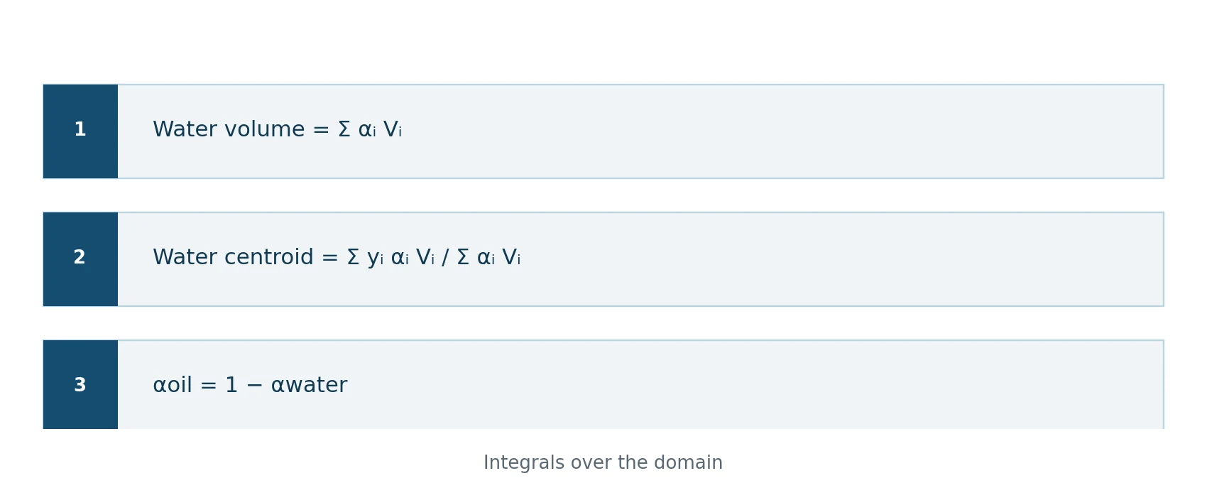
Figure 3 — Integrated phase inventories and volume centroids. For constant-density individual phases, the volume centroid is also their mass centroid.
Deep dive · Package script: phase_metrics.py
It reads a CSV with one row per cell, checks that volumes are positive and that α stays within 0 ± 10⁻⁵ and 1 ± 10⁻⁵ (otherwise it stops, giving the row), rounds only tiny deviations, then prints the volumes and vertical centroids of the two phases and, if --initial-water-volume is given, the relative error. On the synthetic demo_cells_synthetic.csv file (four 0.001 m³ cells) it returns Vw = V2 = 0.002 m³ and centroids 0.1 and 0.3 m, as expected.
python phase_metrics.py cells_t1.csv --alpha alpha.water --volume Volume --y "Points:1" --initial-water-volume 6.4610e-4The value 6.4610·10⁻⁴ m³ is the actual initial inventory (0.044253 m² × 0.0146 m, section 4); it is still best read from the first time of your own run.
#!/usr/bin/env python3
# SPDX-License-Identifier: GPL-3.0-or-later
"""Integrate VOF phase metrics from a ParaView per-cell CSV export.

Required columns: a water fraction, a cell-volume value, cell-centre y.
Specify names using --alpha, --volume, --y (inspect your CSV header).
"""
import argparse,csv,math,sys

def main():
    p=argparse.ArgumentParser(description=__doc__)
    p.add_argument('csv_file')
    p.add_argument('--alpha',default='alpha.water')
    p.add_argument('--volume',default='Volume')
    p.add_argument('--y',default='Points:1')
    p.add_argument('--initial-water-volume',type=float)
    a=p.parse_args()
    vW=vO=weightedW=weightedO=volume=0.0
    min_a,max_a=math.inf,-math.inf
    rows=0
    with open(a.csv_file,encoding='utf-8-sig',newline='') as f:
        reader=csv.DictReader(f)
        if not reader.fieldnames:raise ValueError('Empty CSV or header missing')
        missing=set([a.alpha,a.volume,a.y])-set(reader.fieldnames)
        if missing:raise ValueError(f'Missing columns {sorted(missing)}. Available: {reader.fieldnames}')
        for row in reader:
            try:al=float(row[a.alpha]);vol=float(row[a.volume]);y=float(row[a.y])
            except (ValueError,KeyError) as e:raise ValueError(f'Invalid numeric entry in CSV row {rows+2}') from e
            if not all(map(math.isfinite,[al,vol,y])) or vol <= 0:
                raise ValueError(f'Nonfinite value or non-positive cell volume in row {rows+2}')
            if al < -1e-5 or al > 1.00001:raise ValueError(f'Volume fraction outside tolerance at row {rows+2}: {al}')
            # Keep original fraction for reporting; clamp only tiny roundoff errors.
            al=max(0.0,min(1.0,al))
            w=al*vol;o=(1-al)*vol
            vW+=w;vO+=o;weightedW+=y*w;weightedO+=y*o;volume+=vol
            min_a=min(min_a,al);max_a=max(max_a,al);rows+=1
    if not rows or vW<=0 or vO<=0:raise ValueError('Need nonempty CSV containing positive volumes of both phases')
    print(f'cells,{rows}')
    print(f'domain_volume_m3,{volume:.12g}')
    print(f'water_volume_m3,{vW:.12g}')
    print(f'oil_or_air_volume_m3,{vO:.12g}')
    print(f'water_centroid_y_m,{weightedW/vW:.12g}')
    print(f'oil_or_air_centroid_y_m,{weightedO/vO:.12g}')
    print(f'verify_sum_m3,{vW+vO:.12g}')
    if a.initial_water_volume is not None:
        if a.initial_water_volume<=0:raise ValueError('Initial volume must be >0')
        print(f'water_volume_relative_error,{(vW-a.initial_water_volume)/a.initial_water_volume:.8g}')

if __name__=='__main__':
    try:main()
    except (OSError,ValueError) as e:
        print('ERROR:',e,file=sys.stderr);sys.exit(2)
Deep dive · How large the volume drift should be
The α equation in conservative form with MULES conserves ∫α dV up to the solver tolerance and any boundedness clipping. In a closed domain the expected relative drift is of the order of 10⁻⁶–10⁻⁴ over the whole run; values of 10⁻³ or more signal a problem (too large a step, non-conservative fluxes, inconsistent boundary conditions). In the water-air case water is also conserved as long as it does not leave through the top boundary, while the air volume in the domain is constant only because the fluid is incompressible and the domain is full: the atmosphere boundary lets air in and out.
Export a cell-resolved CSV
Apply Cell Size to the complete mesh in ParaView to obtain Volume; then apply Cell Centers to make cell-centre coordinates available. Use File → Save Data to export a CSV containing alpha.water, the cell volume and vertical cell-centre coordinates. Column labels depend on filters and versions; inspect the CSV header and pass explicit names to the analysis script.
python phase_metrics.py cells_t025.csv --alpha "alpha.water" --volume "Volume" --y "Points:1"If the fields are named alpha.water, CellVolume and y, use --volume CellVolume --y y. The Python 3 utility checks finite positive cell volumes and bounded fractions and returns volumes and centroids. It also runs on Windows with no external packages. Use one row per cell, not an already area-averaged table or arbitrarily sampled points.
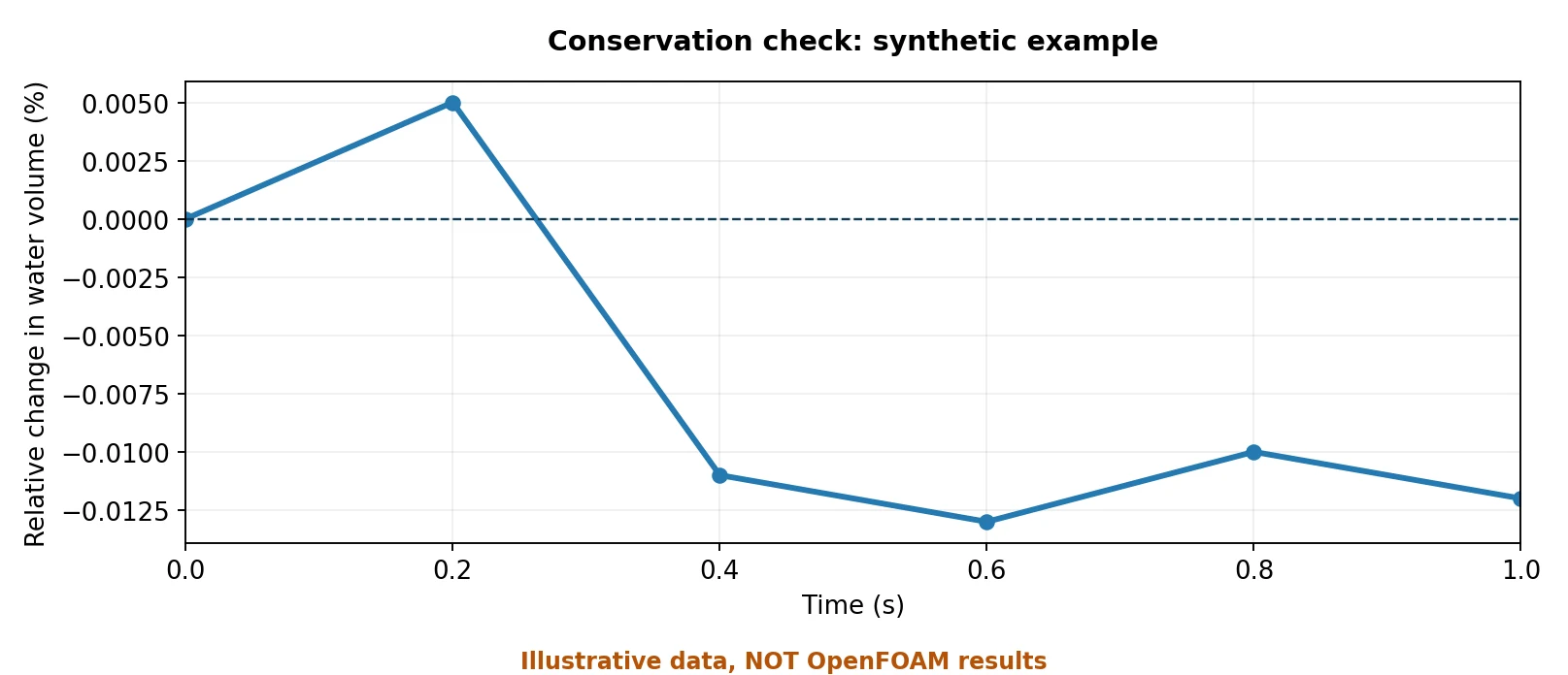
Figure 4 — Synthetic illustration of small phase-inventory drift, not output from the packaged OpenFOAM exercises.
12. Comparisons that are scientifically meaningful
Compare water–oil cases by changing one parameter at a time: water_oil_reference versus water_oil_low_sigma isolates the prescribed surface-tension difference; water_oil_reference versus water_oil_high_nu varies oil viscosity. Water–air serves as a baseline tutorial check but is not an experimentally equivalent separation comparison.
Minimum output fields include: physical time, Vwater, Voil, volume-centroid heights, extrema of alpha.water, maximum Courant number, elapsed time and a clearly defined interface metric. A change in the shape of the α=0.5 isosurface alone does not establish which condition produces more rapid phase separation.
Deep dive · Quantitative metrics to compare the water-oil cases
- Normalised available potential energy: e(t) = (yw(t) − yw,f)/(yw,0 − yw,f), with yw,0 = 0.1452 m and yw,f = 0.0393 m. It is 1 at the start and 0 at full stratification; its decay is the most robust measure of “separation speed”.
- 10 % time: the time at which e(t) falls below 0.1, with uncertainty given by the write interval.
- Level at the stations: the four
interfaceHeightseries must converge to 0.0778 m; their spread measures the amplitude of the residual oscillation. - Interface thickness: vertical distance between the α = 0.05 and 0.95 isolines on a vertical; with compression it should stay at 1–3 cells.
Each metric must be accompanied by the same quantity computed with the doubled mesh (section 8): the difference between the two meshes is the numerical-uncertainty estimate to compare with the effect of the physical parameter. If the difference between reference and low_sigma is smaller than the difference between the two meshes, the correct conclusion is “effect not resolved”, not “no effect”.
Deep dive · Estimating mesh uncertainty with two or three grids
With three meshes at refinement ratio r = 2 and a metric φ (for example the 10 % time or the level at a fixed time) the observed order is p = ln[(φ3 − φ2)/(φ2 − φ1)]/ln r and the extrapolated value is φ1 + (φ1 − φ2)/(rp − 1), with index 1 for the finest mesh. With only two meshes the formal order is assumed (about 1 for limited interfaces) and |φ1 − φ2| is reported as a conservative estimate. The full procedure, with the Grid Convergence Index, is in Guide 4.
13. Troubleshooting
| Symptom | Likely cause | First check |
|---|---|---|
Missing physicalProperties.oil | inconsistent phase/file naming | phaseProperties, file names |
Unknown patch upperWall | mesh or field dictionaries mismatch | constant/polyMesh/boundary, 0/* |
alpha.water outside [0,1] | numerical or exported-data issue | MULES, logs, time step |
| Blurred interface | inadequate spatial/temporal resolution | mesh, Courant, schemes |
| Run ends without useful results | physical or execution setup issue | saved times, fields, balances |
| CSV not recognized | field names do not match defaults | CSV header and --* flags |
| ParaView cannot read case | wrong remote path or session | pvserver and version match |
Do not attribute every unexpected motion to surface tension. Initial conditions, mesh, wall treatment, time step and numerical schemes can all produce similar symptoms.
Deep dive · Other symptoms and their causes
| Symptom | Probable cause | Check |
|---|---|---|
| “Unable to set reference cell for field p” right after start | closed domain without pressure reference | add_pressure_reference.py on a fresh copy |
| pRefPoint “not found” or found on several domains | point outside the domain or on the obstacle | choose an interior point, at mid-thickness (z = 0.0073) |
| phase fraction drifting by more than 10⁻⁴ | step or tolerances | vof_log_summary.py, then maxCo 0.5 |
| maximum velocity not decaying at rest | parasitic currents or sloshing oscillation | UmaxMag over time, finer mesh |
| interfaceHeight constant or zero | station outside the domain or inside the obstacle | coordinates in functions |
| ParaView shows only boundaries | internalMesh not selected | reader “Mesh Regions” panel |
14. Three practical laboratories
Lab A — Water–air dam break. Prepare water_air_reference, run checkMesh and foamRun, save four frames with a fixed alpha.water range 0–1, explain the interface motion and record the maximum Courant number. Compare qualitatively with the official tutorial without claiming quantitative validation.
Lab B — Redistribution of water and oil in a closed container. Run water_oil_reference, calculate initial and final phase inventory, evaluate vertical profiles and display the alpha=0.5 surface. Confirm that the observed arrangement is consistent with density contrast and gravity direction.
Lab C — Physical parameter sensitivity. Compare water_oil_reference, water_oil_low_sigma, and water_oil_high_nu at matched physical times using the same mesh. Plot water centroid and volume inventory and distinguish physical changes from discretisation artifacts.
Deep dive · Expected results of the three experiences
- A: the column collapses and the front reaches the obstacle before 0.1 s; after the impact on the right wall an upward jet forms, followed by a wave travelling back to the left. The maximum Courant stays close to 1 because the step is adjusted; the actual step falls to a few milliseconds in the fastest phases.
- B: water flows along the floor under the oil as a gravity current; the water centroid falls from 0.145 m towards 0.039 m, but within 1 s the process has barely started. The water inventory must stay constant within 10⁻⁴.
- C: the doubled oil viscosity slows the front and damps oscillations sooner; the reduced interfacial tension has a small effect with this mesh (section 3). Report every difference together with the numerical uncertainty estimate.
15. Laboratory record and completion criteria
| Record item | Value |
|---|---|
| OpenFOAM / ParaView versions | … |
| Case identifier and origin | … |
| Mesh size, cell count and dimensions | … |
| Phase densities and viscosities | … |
| Interfacial tension | … |
deltaT, maxCo, maxAlphaCo | … |
| Studied physical time interval | … |
Initial/final Vwater, relative drift | … |
ywater and yoil | … |
| Findings and model limitations | … |
The exercise is complete when independent cases have been prepared safely, at least one simulation has run successfully, logs are preserved, visualisations can be compared, phase balances are reported and uncertainties/limitations are discussed. A visually pleasing image is not sufficient: a useful scientific result must state what the data establish and what they do not establish.
Practical tip · Additional rows for the laboratory sheet
- Actual initial inventory (from the log or
volIntegrate) and nominal box area. - Pressure reference used in the closed cases (
pRefPoint,pRefValue). - Actual
endTimeand value of e(t) at the last time. - Minimum and maximum α over the whole run, with the worst time.
- Doubled-mesh results for at least one metric.
cd "$HOME/cases"
foamVersion > Guide13_cases/OPENFOAM_VERSION.txt 2>&1
tar czf Guide13_cases_$(date +%Y%m%d).tar.gz Guide13_cases
sha256sum Guide13_cases_*.tar.gz > Guide13_cases_SHA256.txt
16. Connection with liquid–liquid extraction
Actual solute extraction from water into an oil phase requires at least one species field in each liquid, phase-dependent diffusivities, partition equilibrium or interfacial transfer kinetics, molar balances and potentially chemical reactions. The VOF model in this guide can help resolve the evolving phase geometry, but it is not itself an extraction model. Guide 13 deliberately focuses on two-phase hydrodynamics.
Deep dive · From VoF to mass transfer between phases
The first step available in OpenFOAM 14 without writing code is phaseScalarTransport: it solves a tracer confined to one phase, transported with that phase’s flux. The damBreakTracer tutorial uses it like this:
// system/functions
#includeFunc phaseScalarTransport(field=tracer.water)
#includeFunc phaseScalarTransport(field=tracer.air, residualAlpha=1e-6)

// system/fvSchemes
div(alphaPhi,tracer) Gauss vanLeer;
Real transfer between phases additionally requires an equilibrium condition at the interface (for example a Henry partition coefficient, coil = K cwater) and continuity of the diffusive flux; with a diffuse interface the concentration jump is handled with the “continuous species transfer” (CST) method, developed for OpenFOAM by Marschall and co-workers (Chem. Eng. Sci. 78, 2012). For drops smaller than the cell one moves to the multiphaseEuler module with interfacial mass-transfer models. These are the topics of Guides 17–18 of the path.
17. Quick commands and official references
# Linux server — only in a fresh Guide 13 workspace
foamVersion
python3 prepare_cases.py --destination "$HOME/cases/Guide13_cases"
bash run_case.sh "$HOME/cases/Guide13_cases/water_air_reference"
head -n 25 "$HOME/cases/Guide13_cases/water_air_reference/log.foamRun"
tail -n 35 "$HOME/cases/Guide13_cases/water_air_reference/log.foamRun"
Primary sources: OpenFOAM Foundation 14 — dam-break user guide; official damBreakLaminar case; Foundation 14 field initialisation; ParaView documentation.
Original guide scripts: GNU GPL v3 or later. Copies of OpenFOAM official tutorials are subject to their original licenses.
Deep dive · Reference reading, with links
- C. W. Hirt, B. D. Nichols, «Volume of fluid (VOF) method for the dynamics of free boundaries», J. Comput. Phys. 39 (1981), doi:10.1016/0021-9991(81)90145-5.
- J. U. Brackbill, D. B. Kothe, C. Zemach, «A continuum method for modeling surface tension», J. Comput. Phys. 100 (1992), doi:10.1016/0021-9991(92)90240-Y.
- S. T. Zalesak, «Fully multidimensional flux-corrected transport algorithms for fluids», J. Comput. Phys. 31 (1979), doi:10.1016/0021-9991(79)90051-2.
- S. S. Deshpande, L. Anumolu, M. F. Trujillo, «Evaluating the performance of the two-phase flow solver interFoam», Comput. Sci. Discov. 5 (2012), doi:10.1088/1749-4699/5/1/014016.
- F. Denner, B. G. M. van Wachem, «Numerical time-step restrictions as a result of capillary waves», J. Comput. Phys. 285 (2015), doi:10.1016/j.jcp.2015.01.021.
- S. Popinet, «Numerical models of surface tension», Annu. Rev. Fluid Mech. 50 (2018), doi:10.1146/annurev-fluid-122316-045034.
- J. C. Martin, W. J. Moyce, «An experimental study of the collapse of liquid columns on a rigid horizontal plane», Phil. Trans. R. Soc. A 244 (1952), doi:10.1098/rsta.1952.0006.
- T. B. Benjamin, «Gravity currents and related phenomena», J. Fluid Mech. 31 (1968), cambridge.org.
- H. Marschall et al., «Numerical simulation of species transfer across fluid interfaces in free-surface flows using OpenFOAM», Chem. Eng. Sci. 78 (2012).
- OpenFOAM Foundation 14 user guide — dam break.
Deep dive · The OpenFOAM 14 source files cited in the boxes
- tutorials/incompressibleVoF/damBreakLaminar — the starting case
- applications/modules/incompressibleVoF — the solver module
- findRefCell.C — the pressure-reference message
- sloshingTank2D/system/fvSolution — pRefPoint in a closed tank
- damBreak3D/system/fvSchemes — MPLIC scheme
- interfaceHeight.H — interface height
- tutorials/incompressibleVoF/damBreakTracer — phase tracer
- functionObjectList.C — reading of system/functions (header required)
Deep dive · Package files and additional scripts of this article
| File | Where it is reproduced | Status |
|---|---|---|
scripts/prepare_cases.py | section 5 | from the package, tested on the real tutorial |
scripts/run_case.sh | section 7 | from the package |
scripts/phase_metrics.py | section 11 | from the package, tested on the synthetic CSV |
add_pressure_reference.py | section 5 | additional, required fix for the closed cases |
functions_guide13 | section 7 | additional |
vof_estimates.py | section 3 | additional |
vof_log_summary.py | section 8 | additional, tested |
vof_equilibrium.py | section 9 | additional, tested |
The examples/demo_cells_synthetic.csv file contains four synthetic rows (two water cells at y = 0.1 m and two oil cells at y = 0.3 m): it only serves to test the parser, it is not a CFD result. All new scripts are released under GPL-3.0-or-later.
Practical tip · Reading the function-object results
cd "$HOME/cases/Guide13_cases/water_oil_reference/postProcessing"
ls -R | head -n 20
tail -n 3 "volIntegrate(alpha.water)/0/volFieldValue.dat"
tail -n 3 interfaceHeight1/0/*.dat
tail -n 3 UmaxMag/0/*.dat
Each file starts with comment lines (#) describing the columns; interfaceHeight writes one file with the heights (above the station and above the lowest boundary) and one with the positions of the interface points. Columns are read with the same approach as the .dat scripts of Guide 12 or directly in a spreadsheet, ignoring the comment lines.
Related guides: Linux server from Windows, monitoring and convergence, ParaView for quantitative analysis, verification and validation, parameter sweeps, mesh generation and quality checks, boundary conditions and physical models, transient simulations, turbulence and RANS models, heat transfer and natural convection, conjugate heat transfer, species transport, diffusion and mixing and the Learning OpenFOAM 14 path.
Deep dive · Package files: complete data and examples
Full text of the synthetic file examples/demo_cells_synthetic.csv (four cells, illustrative data, not CFD) used to test phase_metrics.py.
alpha.water,Volume,Points:1
1,0.001,0.1
1,0.001,0.1
0,0.001,0.3
0,0.001,0.3
Download: scripts and files of the guide
The archive OpenFOAM14_Guida13_script.zip (25 kB compressed, 9 files) contains every script and data file reproduced or cited in this article, with the same content as the boxes: the scripts/, examples/ and similar folders hold the guide package files, extra/ the additional scripts and files presented in the deep dives. README_IT_EN.txt lists the contents with SHA-256 checksums; files marked SYNTHETIC are illustrative data, not CFD results. Licence GNU GPL v3 or later (COPYING_GPLv3.txt).
Important: after prepare_cases.py and before run_case.sh on the water-oil cases run python3 extra/add_pressure_reference.py "$HOME/cases/Guide13_cases" (section 5).
Archive contents:
examples/demo_cells_synthetic.csv— SYNTHETIC / illustrative data, not CFD results (5 lines)extra/add_pressure_reference.py— Add a pressure reference to the closed water-oil cases of Guide 13.extra/functions_guide13— system/functions file for OpenFOAM 14 (with FoamFile header)extra/vof_equilibrium.py— Initial inventory and stratified end state of the damBreakLaminar geometry.extra/vof_estimates.py— Scale analysis for the Guide 13 VOF cases (damBreakLaminar geometry).extra/vof_log_summary.py— Summarise an OpenFOAM 14 incompressibleVoF log (log.foamRun).scripts/phase_metrics.py— Integrate VOF phase metrics from a ParaView per-cell CSV export.scripts/prepare_cases.py— Prepare safe, independent OpenFOAM Foundation 14 VOF tutorial variants.scripts/run_case.sh— Run one fresh Guide 13 case without deleting or overwriting existing results.