

OpenFOAM: species transport, diffusion and mixing
Twelfth guide of the Learning OpenFOAM 14 path and the fourth and last of the “Turbulence, heat and mass” module of the advanced course, after those on server and transfers, monitoring and convergence, quantitative analysis with ParaView, verification and validation, parameter sweeps, mesh generation, boundary conditions and models, transient simulations, turbulence and RANS models, heat transfer and conjugate heat transfer. This one tackles passive tracer transport: advection, diffusion, Péclet number, numerical diffusion and mixing, with the scalarTransport function object and the functions solver on the official pitzDailyScalarTransport case. The deep-dive and practical-tip boxes open with a click: they contain every package script, the actual tutorial data read from its files (flow rate, volume, residence time, turbulent viscosity), a reading of the OpenFOAM 14 source code, the fix required for the system/functions file prepared by the scripts to be actually read, a monitoring file for inventory, flows and cup-mixing concentration, six additional tested scripts (estimates, front metrics, the Ogata–Banks analytical solution, linearity test, tracer balance, residence time distribution) and linked bibliographic references.
Practical OpenFOAM series · OpenFOAM Foundation 14 · Linux server + Windows client
Purpose. Model and interpret passive-tracer transport, separating advection, physical diffusion, and numerical dispersion. Prepare four independent cases, extract quantitative profiles using ParaView and compare them on Windows.
Scope. This is a single-phase flow with a passive scalar that does not alter density, viscosity, velocity or temperature. It does not model two immiscible liquids, a VOF interface, or reactions. The selected diffusivities are teaching values, not typical molecular diffusion coefficients in water.
Prerequisites: Guides 1–4 (SSH/FileZilla/ParaView and verification), Guides 5 and 8 (campaigns and transient runs), basic species-balance concepts. Windows editor: Notepad++; no Visual Studio Code required.
1. Learning objectives
After completing this guide you should be able to define a dimensionless scalar field, execute OpenFOAM Foundation 14’s functions solver with scalarTransport, choose compatible boundary conditions, compare convective and diffusive effects, quantify scalar profiles, identify numerical artifacts and archive a reproducible report.
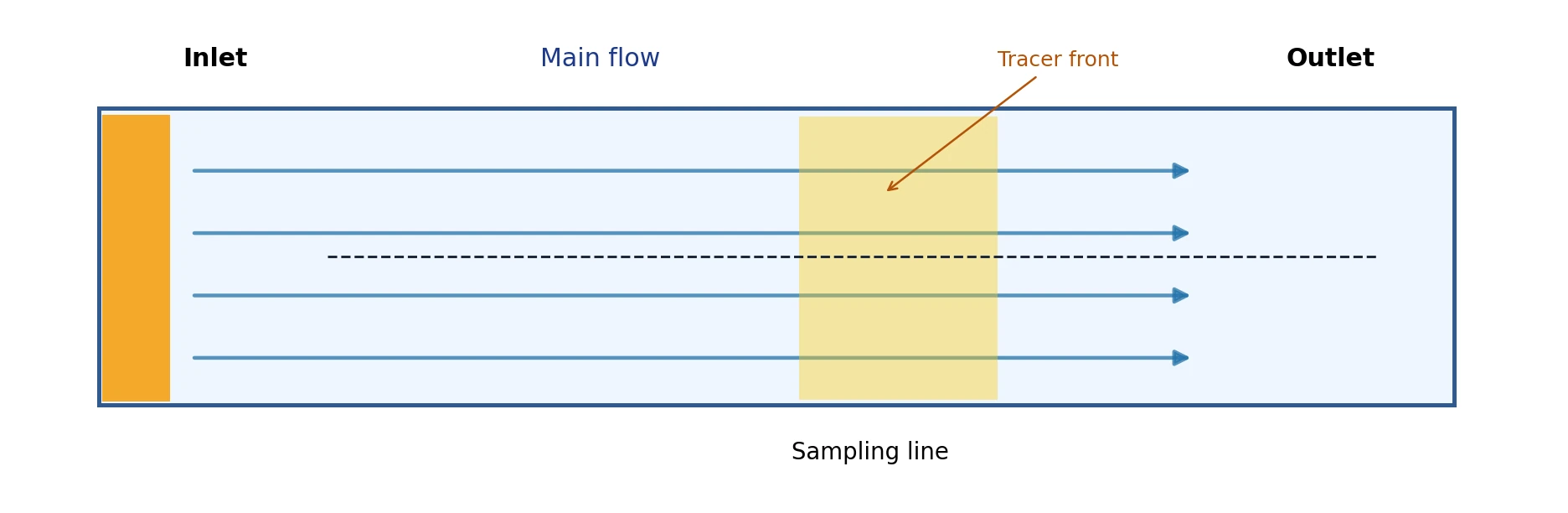
Figure 1 — Original conceptual drawing: a tracer front advects downstream while diffusion smooths the gradient. Not an OpenFOAM result.
Deep dive · The equation OpenFOAM 14 actually solves, line by line
The scalarTransport function object is defined in scalarTransport.C. For a volumetric flux (phi in m³/s, incompressible case) and without MULES, at every time step it assembles and solves:
fvm::ddt(C) + fvm::div(phi, C, "div(phi,C)")
  - fvm::laplacian(DC, C, "laplacian(DC,C)")
 == fvModels.source(C)

DC = D                          (diffusivity constant)
DC = alphal*nu + alphat*nut     (diffusivity viscosity)
no diffusion term (diffusivity none)- The diffusion scheme name is
laplacian(DC,C): the diffusivity field is called “D” followed by the field name. Here it is covered bydefault Gauss linear corrected; withdefault noneit would have to be declared explicitly. - The number of corrections
nCorr(ornCorrectors) is read from the solver dictionary ofCinfvSolutionand defaults to 0: the equation is solved once per step. With a linear scheme nothing else is needed; with limited (non-linear) schemes 1–2 corrections make the result less dependent on the previous-step value. - Any sources are added through
constant/fvModelsand constraints (for example a bound) throughsystem/fvConstraints: the code calls them explicitly. This is the way to a decaying tracer or a localised source without writing code. - The
schemesFieldandsolverFieldentries reuse the schemes and solver of another field;phiandrhochange the names of the flux and density fields.
Defaults of the etc/caseDicts/functions/solvers/scalarTransport configuration: diffusivity viscosity; alphal 1; alphat 1; writeControl writeTime;. In the guide the #includeFunc arguments replace the diffusivity with constant and the value D.
Deep dive · What the “functions” solver does (and does not do)
The applications/modules/functions module instantiates the sub-solver named in subSolver (here incompressibleFluid) only to build the fields and physical models, then runs only the function objects in the time loop. From the source code:
- all sub-solver steps (momentum predictor, pressure corrector, turbulence) are empty:
U,phi,k,epsilon,nutstay as read from0/(“frozen” field); subSolverTime 0makes the sub-solver fields be read from the0directory even when restarting from a later time;- the sub-solver fields are set to
NO_WRITE: onlyCappears in the time directories (plus fields written by other function objects). In ParaViewUexists only at time 0; maxDeltaT()returns an infinite value andcontrolDicthas noadjustTimeStep: the step stays fixed atdeltaT 0.0001and the Courant number is not controlled (box in section 3).
Since the sub-solver builds the kEpsilon turbulence model, nu and nut are available: the diffusivity viscosity option and the PecletNo function object also work with the frozen field.
Practical tip · The case data sheet, measured on the files
| Quantity | Value | Source |
|---|---|---|
| cells | 12 225 | resources/blockMesh/pitzDaily mesh |
| domain volume (1 mm thick) | 1.452·10⁻⁵ m³ | blockMesh vertices |
flow rate Q (sum of phi at the inlet) | 2.540·10⁻⁴ m³/s | 0/phi |
| space time τ = V/Q | 57.1 ms | computed |
| U at the inlet, ν | 10 m/s; 1·10⁻⁵ m²/s | 0/U, constant/physicalProperties |
| Re = U h/ν (h = 25.4 mm) | 25 400 | turbulent flow, kEpsilon model |
nut: median, mean, maximum | 8.3·10⁻⁴; 1.55·10⁻³; 5.2·10⁻³ m²/s | 0/nut |
| minimum flux on an outlet face | +6.2·10⁻⁷ m³/s (no backflow) | 0/phi |
| deltaT, endTime, writeInterval | 1·10⁻⁴ s; 0.2 s; 50 steps = 5 ms | system/controlDict |
The sum of the inlet (−2.53999·10⁻⁴) and outlet (+2.54008·10⁻⁴ m³/s) fluxes agrees within 3·10⁻⁵ in relative terms: the supplied phi field is conservative, a prerequisite for any tracer balance. All 57 outlet fluxes are positive, so the zeroGradient condition on C at the outlet never receives inflow.
2. Governing transport equation
For incompressible fluid velocity U, dimensionless tracer C, and constant diffusivity D, with no sources:

The conservative total tracer flux is:
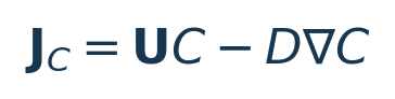
Here C is dimensionless (a normalized tracer fraction or label), D has units m²/s, velocity m/s and J_C m/s. Thus ∫Ω C dV has units m³: it is a normalized inventory, not solute mass. A mass concentration (kg/m³) and a mass fraction require their own consistent inventory and flux definitions, including density where appropriate.
Optional refresher — Advection versus diffusion. Advection moves material with the fluid; molecular diffusion redistributes it along a concentration gradient. Neither process is a synonym for mixing between immiscible phases.
Deep dive · Maximum principle and steady solution: two free tests
Without sources, with 0 ≤ C ≤ 1 on the boundary and in the initial condition, the exact solution of the advection-diffusion equation satisfies 0 ≤ C ≤ 1 everywhere and at all times (maximum principle). Any value below 0 or above 1 is therefore a numerical error (typically oscillations of an unbounded scheme), not physics. For D_half_inlet the upper bound is 0.5.
With an inlet at C = 1, zeroGradient walls and outlet and no source, the only steady solution is C ≡ 1 in the whole domain, regardless of D. Practical consequences: (1) cases A, B and C all converge to the same field and differences exist only in the transient; (2) the inventory ∫C dV must tend to the domain volume, 1.452·10⁻⁵ m³; (3) if regions with C < 1 remain after many residence times, they are slow-exchange regions (the recirculation bubble behind the step), not an error.
Deep dive · From laminar tracer to turbulent closure: Sc and Sct
In a Reynolds-averaged turbulent flow the turbulent flux ⟨u′c′⟩ appears, closed with the gradient hypothesis ⟨u′c′⟩ = −(νt/Sct) ∇C̄. The mean equation therefore has an effective diffusivity Deff = ν/Sc + νt/Sct, which is exactly the diffusivity viscosity option with alphal = 1/Sc and alphat = 1/Sct.
The turbulent Schmidt number is not universal: the review by Tominaga and Stathopoulos (2007) reports optimal values between 0.2 and 1.3 depending on the flow, with 0.7 as the most common choice. The value must therefore be declared and, when possible, varied in a sensitivity study.
A figure that changes how the campaign is read. In the tutorial 0/nut field νt has a median of 8.3·10⁻⁴ m²/s and a maximum of 5.2·10⁻³ m²/s: with Sct = 0.7 the turbulent diffusivity is about 1.2·10⁻³ m²/s (median) and up to 7.4·10⁻³ m²/s in the mixing layer. The guide’s “teaching” diffusivities (10⁻³–5·10⁻² m²/s) are therefore of the same order as the turbulent diffusivity of this flow, while the molecular diffusivity of a gas (~10⁻⁵ m²/s) would be two to three orders of magnitude smaller. A fifth, physically more consistent case is:
// system/functions of a copy E_turbulent (Sc = 1, Sc_t = 0.7)
#includeFunc scalarTransport(C, diffusivity=viscosity, alphal=1, alphat=1.43)
Prepare it by copying A_reference into a new folder before running and changing only that line (keeping the FoamFile header, section 5).
Practical tip · From the normalised inventory to a mass
The case is two-dimensional with a 1 mm thickness: volIntegrate(C) returns m³ referred to that thickness. For a reference concentration cref (kg/m³) the solute mass is m = cref·∫C dV; per metre of depth multiply by 1000. Likewise the advective flow Σφ C (m³/s) becomes a mass flow rate when multiplied by cref. With a mass fraction Y one would need ∫ρY dV instead, which in a constant-density flow is ρ·∫Y dV.
3. Time scales and the Péclet number
A basic comparison uses:

Choose U and L to match the actual flow and physical effect of interest. Large Pe means advection is more influential; small Pe makes diffusion more influential. The Courant number is a separate indicator of time resolution on the mesh. In turbulent flow distinguish molecular diffusivity from an effective diffusivity, possibly linked to eddy viscosity and turbulent Schmidt number.
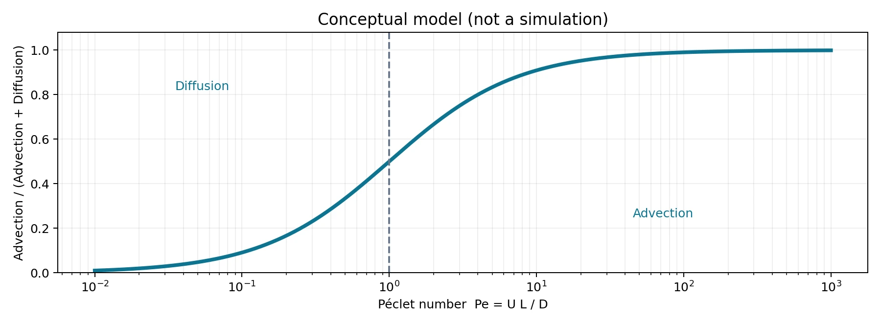
Figure 2 — A conceptual nondimensional illustration, not a CFD data curve.
Deep dive · The campaign numbers (tracer_estimates.py script)
Cell spacings come from the gradings in resources/blockMesh/pitzDaily (main block: 180 cells over 206 mm with ratio 4).
| D (m²/s) | Peh = U h/D | tdiff = h²/D | cell Pe (U = 10 m/s, Δx = 0.53 mm) | cell Pe (U = 5 m/s, Δx = 1.4 mm) | D/ν |
|---|---|---|---|---|---|
| 0.001 | 254 | 0.645 s | 5.3 | 7.0 | 100 |
| 0.01 | 25.4 | 0.065 s | 0.53 | 0.70 | 1000 |
| 0.05 | 5.1 | 0.013 s | 0.11 | 0.14 | 5000 |
- Crossing time of the inlet channel (20.6 mm at 10 m/s): 2.1 ms; mean velocity after the 2:1 expansion about 5 m/s.
- Courant number with the tutorial step: 1.89 on the shortest cells near the step, 0.36 downstream.
- The ratio D/ν = 1/Sc is 100–5000: Sc = 10⁻²–10⁻⁴, values no real fluid has (gases ≈ 0.7–1, liquids ≈ 10²–10³). This is another confirmation that D must be read as an effective, not molecular, diffusivity.
#!/usr/bin/env python3
# SPDX-License-Identifier: GPL-3.0-or-later
"""Order-of-magnitude estimates for the Guide 12 passive-tracer campaign.

Geometry and spacing come from the OpenFOAM 14 resource
tutorials/resources/blockMesh/pitzDaily (units mm, 1 mm thick, 12 225 cells).
Inlet velocity 10 m/s, nu = 1e-5 m2/s, deltaT = 1e-4 s, endTime = 0.2 s.
The numbers help to choose sampling times and to judge numerical diffusion;
they are not CFD results.
"""
import argparse
import math


def graded(length, n, ratio):
    """First and last cell of a simpleGrading block (ratio = last/first)."""
    r = ratio ** (1.0 / (n - 1))
    first = length * (1 - r) / (1 - r ** n)
    return first, first * r ** (n - 1)


def main():
    p = argparse.ArgumentParser(description=__doc__)
    p.add_argument('--U', type=float, default=10.0, help='inlet velocity [m/s]')
    p.add_argument('--h', type=float, default=0.0254, help='step / inlet height [m]')
    p.add_argument('--dt', type=float, default=1e-4, help='time step [s]')
    p.add_argument('--D', type=float, nargs='*', default=[0.001, 0.01, 0.05], help='diffusivities [m2/s]')
    p.add_argument('--nu', type=float, default=1e-5, help='kinematic viscosity [m2/s]')
    a = p.parse_args()

    # Areas in mm2 of the 2D domain (inlet channel, expansion, tapered outlet), depth 1 mm.
    area_mm2 = 20.6 * 25.4 + 206.0 * 50.8 + 84.0 * (50.8 + 33.2) / 2.0
    volume = area_mm2 * 1e-9                      # m3
    q_in = a.U * a.h * 1e-3                       # m3/s through a 1 mm deep inlet
    print(f'Domain volume (1 mm deep) = {volume:.4e} m3, inlet flow = {q_in:.4e} m3/s')
    print(f'Space time V/Q (mean fill time) = {volume / q_in * 1000:.1f} ms')
    print(f'Time to cross the 20.6 mm inlet channel at U = {a.U} m/s: {0.0206 / a.U * 1000:.2f} ms')
    print(f'Mean velocity after the 2:1 expansion ~ {a.U / 2:.1f} m/s')
    print(f'Re based on h = {a.U * a.h / a.nu:.0f}')
    cells = {'inlet block x (grading 0.5)': graded(20.6e-3, 18, 0.5),
             'main block x (grading 4)': graded(206e-3, 180, 4.0),
             'outlet block x (grading 2.5)': graded(84e-3, 25, 2.5)}
    for name, (d0, d1) in cells.items():
        print(f'{name}: first {d0 * 1000:.2f} mm, last {d1 * 1000:.2f} mm')
    dx_min = cells['main block x (grading 4)'][0]
    print(f'Courant at the step (U = {a.U} m/s, dx = {dx_min * 1000:.2f} mm) = {a.U * a.dt / dx_min:.2f}')
    print(f'Courant downstream (U = {a.U / 2:.1f} m/s, dx = 1.4 mm) = {a.U / 2 * a.dt / 1.4e-3:.2f}')
    print('D [m2/s]   Pe_h=Uh/D   t_diff=h^2/D [s]   cell Pe (U, dx_min)   cell Pe (U/2, 1.4 mm)   D/nu')
    for D in a.D:
        print(f'{D:<9g}  {a.U * a.h / D:9.1f}   {a.h ** 2 / D:13.4f}      {a.U * dx_min / D:12.2f}        {a.U / 2 * 1.4e-3 / D:12.2f}        {D / a.nu:7.0f}')
    print('Molecular diffusivity of small solutes in water ~1e-9 m2/s: Pe_h ~ %.1e, Sc = nu_water/D ~ 1000' % (a.U * a.h / 1e-9))


if __name__ == '__main__':
    main()
Deep dive · Numerical diffusion: how large it is in the tutorial case
Modified-equation analysis shows that the implicit Euler time scheme, applied to convective transport, adds a numerical diffusivity of the order of
D_num,t ≈ U² Δt / 2| Region | U | Dnum,t (Δt = 10⁻⁴ s) | comparison |
|---|---|---|---|
| inlet channel | 10 m/s | 5·10⁻³ m²/s | 5 times D of case B, half of D of case A |
| downstream of the expansion | 5 m/s | 1.25·10⁻³ m²/s | larger than D of case B |
The linearUpwind spatial scheme is second order and its leading error is dispersive (oscillations), not diffusive; a first-order upwind scheme would instead add U·Δx/2 ≈ 2.6–3.5·10⁻³ m²/s. Conclusion: in case B the apparent diffusion is dominated by the time discretisation, and the A/B/C comparison partly measures numerics. Verifiable remedies:
// system/fvSchemes - second-order time scheme (no leading-order numerical diffusion)
ddtSchemes
{
    default         backward;
}

// system/controlDict - Courant below 1 also on the shortest cells
deltaT          2.5e-05;
writeInterval   200;      // still one write every 5 ms
Run B with Δt = 10⁻⁴, 5·10⁻⁵ and 2.5·10⁻⁵ s (Euler) and then with backward, and compare the front thickness with the front_metrics.py script (section 9): the change between steps estimates the time error. Reference: Moukalled, Mangani, Darwish, The Finite Volume Method in CFD, Springer 2016, chapters on convection schemes and modified-equation analysis.
Deep dive · Cell Péclet number and scheme boundedness
For a central scheme the steady discrete solution stays free of oscillations only if the cell Péclet number PeΔ = U Δx/D does not exceed 2 (Patankar, 1980). In case B PeΔ = 5–7: without a limiter small over- and undershoots on the front are expected. TVD schemes (doi:10.1137/0721062, Sweby 1984) remove oscillations by locally reducing the order; the QUICK scheme of doi:10.1016/0045-7825(79)90034-3 (Leonard 1979) is third order but unbounded.
The OpenFOAM 14 PecletNo function object (PecletNo.C) computes |φ|/(|Sf| δ νeff) on the faces: it uses the effective viscosity, so it is a “momentum” Péclet number. For the tracer at constant D the cell Péclet number is PecletNo·νeff/D. Example of after-the-fact use:
foamPostProcess -solver incompressibleFluid -time 0 -func "PecletNo"
foamPostProcess -solver incompressibleFluid -time 0 -func "CourantNo"
Deep dive · Taylor–Aris dispersion: when apparent diffusion is not D
In a duct with a non-uniform velocity profile, the combination of shear and transverse diffusion spreads the front far more than D. For times long compared with a²/D the cross-section-averaged front behaves as diffusion with an effective coefficient:
pipe (Poiseuille, radius a):           D_eff = D + a² Ū² / (48 D)
parallel plates (Poiseuille, gap h):   D_eff = D + h² Ū² / (210 D)
Microfluidic example: a = 50 µm, Ū = 1 mm/s, D = 10⁻⁹ m²/s give Deff ≈ 53 D. Note that D is in the denominator: a smaller diffusivity produces larger dispersion. The origins are doi:10.1098/rspa.1953.0139 (Taylor 1953) and doi:10.1098/rspa.1956.0065 (Aris 1956, method of moments). In the pitzDaily case the turbulent profile and the recirculation bubble produce a similar dispersion: this is why the guide warns against attributing all apparent diffusion to D.
4. The official OpenFOAM 14 case
We start from the official tutorial:
$FOAM_TUTORIALS/incompressibleFluid/pitzDailyScalarTransport
├── 0/                 T, U, phi, turbulence fields
├── constant/          momentumTransport, physicalProperties
├── system/            controlDict, functions, fvSchemes, fvSolution
└── Allrun
The distributed tutorial includes existing velocity/flux data in 0/U and 0/phi. Its Allrun script generates a compatible mesh using the Foundation resource resources/blockMesh/pitzDaily. These fields must not be combined with an unrelated mesh. In the official tutorial the transported field is named T and declared with temperature dimensions. This guide creates a separate dimensionless field C and changes the solver configuration to evolve C instead; it leaves the original T in the new copies as unchanged provenance data.
The original system/functions also includes a custom mixingQualityCheck coded function object that can stop execution based on mean(T)/max(T). This criterion is unsuitable for standardized fixed-time comparisons, so our new copies replace that configuration with a single scalarTransport(C, ...) function object. No installed tutorial files are changed.
Authoritative references: OpenFOAM-14 pitzDailyScalarTransport; Foundation 14 scalarTransport API.
Deep dive · The tutorial, file by file
| File | Relevant content |
|---|---|
system/controlDict | solver functions; subSolver incompressibleFluid; subSolverTime 0; startFrom latestTime; endTime 0.2; deltaT 0.0001; writeControl timeStep; writeInterval 50; writeFormat ascii; |
system/functions | #includeFunc scalarTransport(T, diffusivity=constant, D = 0.01) plus the coded object mixingQualityCheck |
system/fvSchemes | ddtSchemes default Euler; div(phi,T) Gauss linearUpwind grad(T); laplacianSchemes default Gauss linear corrected; |
system/fvSolution | T { solver PBiCGStab; preconditioner DILU; tolerance 1e-06; relTol 0; } and PIMPLE with 0 non-orthogonal correctors |
constant/momentumTransport | simulationType RAS; model kEpsilon; |
constant/physicalProperties | viscosityModel constant; nu 1e-05; |
0/U | inlet fixedValue (10 0 0), outlet zeroGradient, walls noSlip |
0/phi | face fluxes of the precomputed field (24 170 internal faces) |
0/T | dimensions [temperature]; internalField uniform 0; inlet 1 |
Allrun | runApplication blockMesh -dict $FOAM_TUTORIALS/resources/blockMesh/pitzDaily; runApplication foamRun |
Source: tutorials/incompressibleFluid/pitzDailyScalarTransport and tutorials/resources/blockMesh/pitzDaily.
Deep dive · What mixingQualityCheck did and why it is removed
The coded object computes at every step mixingQuality = mean(T)/max(T), with a volume-weighted mean, and calls writeAndEnd() when it exceeds 0.9. Since max(T) = 1 as soon as the tracer enters, the criterion is equivalent to “inventory/volume > 0.9”: the run would stop at different times for different D, making a fixed-time comparison impossible. Moreover a coded object is compiled at start-up: it needs a working C++ compiler on the server and writes into the case’s dynamicCode folder.
The same quantity is obtained without code using #includeFunc volAverage(C) (volume average) and #includeFunc cellMax(C), which do not stop the run.
Practical tip · Geometry coordinates for choosing sampling lines
From the resources/blockMesh/pitzDaily file (units mm, converted here to metres):
| Region | x (m) | y (m) |
|---|---|---|
| inlet channel | −0.0206 … 0 | 0 … 0.0254 |
| step and main chamber | 0 … 0.206 | −0.0254 … 0.0254 |
| converging outlet section | 0.206 … 0.290 | from ±0.0254 to ±0.0166 |
| thickness | — | z = −0.0005 … 0.0005 |
- Jet line: from (−0.02, 0.0127, 0) to (0.289, 0.0127, 0), the extension of the inlet channel axis.
- Line in the recirculation bubble: from (0.001, −0.0127, 0) to (0.205, −0.0127, 0), below the step.
- Cross-section: from (0.1, −0.0253, 0) to (0.1, 0.0253, 0).
5. Key dictionaries and the new 0/C field
The new volScalarField declares object C with:
dimensions      [0 0 0 0 0 0 0];
internalField   uniform 0;

boundaryField
{
    inlet        { type fixedValue; value uniform 1; }
    outlet       { type zeroGradient; }
    upperWall    { type zeroGradient; }
    lowerWall    { type zeroGradient; }
    frontAndBack { type empty; }
}
Patch names must match the mesh; empty is specific to this nominally two-dimensional setup. The preparation script also modifies:
// system/functions
#includeFunc scalarTransport(C, diffusivity=constant, D = 0.01)

// system/fvSchemes (under divSchemes)
div(phi,C)      Gauss linearUpwind grad(C);

// system/fvSolution (under solvers)
C
{
    solver          PBiCGStab;
    preconditioner  DILU;
    tolerance       1e-06;
    relTol          0;
}
We retain system/controlDict entries including solver functions;, subSolver incompressibleFluid;, subSolverTime 0;, deltaT 0.0001; and endTime 0.2;. The linearUpwind scheme does not automatically guarantee 0 ≤ C ≤ 1; examine minima and maxima and consider a suitably limited scheme only after checking its Foundation 14 support and documenting the change.
Optional refresher — Dimensions are part of the model. Setting [0 0 0 0 0 0 0] is a scientific statement about the tracer. The tutorial’s original temperature-like T should never be relabeled as concentration without checking the physical dimensions and equations.
Deep dive · WARNING: without a FoamFile header the functions file is ignored
The package script writes system/functions with only two lines (a comment and #includeFunc), without the FoamFile header. In OpenFOAM 14 the file is read by functionObjectList::readFunctionsDict, which accepts it only if headerOk() is true, i.e. if the header exists and is of dictionary class. Otherwise the file is skipped without an error: the functions solver runs to endTime with no function object at all, and the C field is never solved or written.
Symptoms: the log contains no scalarTransport execute: or Solving for C lines; time directories contain no C; the four cases are identical. Quick check after a run:
grep -c "Solving for C" A_reference/log.foamRun     # expected: 2000 (one solve per step)
ls A_reference/0.1                                    # expected: C
Fix, to apply to the freshly prepared copies and before run_campaign.sh: the additional add_foamfile_header.py script adds the header to the four files, keeps the original as system/functions.noheader, refuses cases already run and never touches the installed tutorial. It was tested on real copies prepared from the OpenFOAM 14 tutorial (four headers added, original content unchanged below the header).
python3 scripts/prepare_campaign.py --output "$HOME/cases/guide12_species_01"
python3 add_foamfile_header.py "$HOME/cases/guide12_species_01"
head -n 16 "$HOME/cases/guide12_species_01/A_reference/system/functions"
#!/usr/bin/env python3
# SPDX-License-Identifier: GPL-3.0-or-later
"""Add the FoamFile header to system/functions in the Guide 12 case copies.
OpenFOAM 14 reads system/functions only if the file starts with a FoamFile
header (functionObjectList::readFunctionsDict -> IOobject::headerOk()); a
headerless file is silently ignored and scalarTransport(C) would not run.
The tool works only on prepared copies that have not been run yet: it refuses
cases with log.foamRun, keeps the original as system/functions.noheader and
never touches the installed tutorial.
"""
import argparse
import re
from pathlib import Path
import sys
HEADER = '''/*--------------------------------*- C++ -*----------------------------------*\\
Guide 12 - functions file with the header required by OpenFOAM 14
\\*---------------------------------------------------------------------------*/
FoamFile
{
format ascii;
class dictionary;
location "system";
object functions;
}
'''
CASES = ('A_reference', 'B_low_diffusivity', 'C_high_diffusivity', 'D_half_inlet')
def has_header(text):
"""True if the first token after C/C++ comments is the keyword FoamFile."""
body = re.sub(r'/\*.*?\*/', ' ', text, flags=re.S)
body = re.sub(r'//[^\n]*', ' ', body)
return body.split()[:1] == ['FoamFile']
def main():
p = argparse.ArgumentParser(description=__doc__)
p.add_argument('campaign', type=Path, help='folder created by prepare_campaign.py')
a = p.parse_args()
root = a.campaign.expanduser().resolve()
if not (root / 'case_parameters.csv').is_file():
p.error('Not a Guide 12 campaign folder (case_parameters.csv missing)')
for name in CASES:
case = root / name
f = case / 'system' / 'functions'
if not f.is_file():
p.error(f'Missing {f}')
if (case / 'log.foamRun').exists():
p.error(f'{name} has already been run; prepare a new campaign instead')
text = f.read_text(encoding='utf-8')
if has_header(text):
print(f'{name}: header already present, unchanged')
continue
backup = f.with_name('functions.noheader')
if backup.exists():
p.error(f'{backup} already exists; refusing to overwrite it')
backup.write_text(text, encoding='utf-8')
f.write_text(HEADER + text, encoding='utf-8')
print(f'{name}: header added (original kept in {backup.name})')
if __name__ == '__main__':
try:
main()
except OSError as exc:
sys.exit(f'ERROR: {exc}')Deep dive · A complete functions file to measure during the run
The following file, valid for OpenFOAM 14, replaces the minimal one in a copy not yet run (adapt the value of D to the case). Besides the transport it computes at every step the inventory, the minimum and maximum of C, the advective flow Σφ C at the inlet (negative) and outlet (positive) and the cup-mixing concentration at the outlet Σφ C/Σφ. The data go to postProcessing/<name>/0/*.dat and are the inputs of the scripts in sections 10–12.
/*--------------------------------*- C++ -*----------------------------------*\
  Guide 12 - functions file for ONE prepared case (here A_reference, D = 0.01)
  The FoamFile header is required: without it OpenFOAM 14 ignores the file.
\*---------------------------------------------------------------------------*/
FoamFile
{
    format      ascii;
    class       dictionary;
    location    "system";
    object      functions;
}

// Passive dimensionless tracer (keep the D value of the case!)
#includeFunc scalarTransport(C, diffusivity=constant, D = 0.01)

// Inventory I(t) = integral of C over the domain [m3] and extreme values
#includeFunc volIntegrate(C)
#includeFunc cellMin(C)
#includeFunc cellMax(C)

// Advective tracer flow sum(phi*C) [m3/s]: negative at the inlet, positive at the outlet
CflowInlet
{
    type            surfaceFieldValue;
    libs            ("libfieldFunctionObjects.so");
    writeControl    timeStep;
    writeInterval   1;
    log             yes;
    writeFields     false;
    patch           inlet;
    operation       sum;
    weightField     phi;
    fields          (C);
}

CflowOutlet
{
    type            surfaceFieldValue;
    libs            ("libfieldFunctionObjects.so");
    writeControl    timeStep;
    writeInterval   1;
    log             yes;
    writeFields     false;
    patch           outlet;
    operation       sum;
    weightField     phi;
    fields          (C);
}

// Flow-weighted (cup-mixing) outlet concentration sum(phi*C)/sum(phi)
CbulkOutlet
{
    type            surfaceFieldValue;
    libs            ("libfieldFunctionObjects.so");
    writeControl    timeStep;
    writeInterval   1;
    log             yes;
    writeFields     false;
    patch           outlet;
    operation       average;
    weightField     phi;
    fields          (C);
}

// ************************************************************************* //
# install it in the four prepared copies, with the D of each case (copies not yet run)
ROOT="$HOME/cases/guide12_species_01"
for spec in A_reference:0.01 B_low_diffusivity:0.001 C_high_diffusivity:0.05 D_half_inlet:0.01; do
n=${spec%%:*}; d=${spec##*:}
[ -e "$ROOT/$n/log.foamRun" ] && { echo "$n already run, skipped"; continue; }
cp -n "$ROOT/$n/system/functions" "$ROOT/$n/system/functions.minimal"
sed "s/D = 0.01)/D = $d)/" functions_guide12 > "$ROOT/$n/system/functions"
grep -H "scalarTransport" "$ROOT/$n/system/functions"
doneThe sed only changes the scalarTransport line (the only one containing “D = 0.01)”); the final grep shows the value actually installed in each case, to compare with case_parameters.csv.
Deep dive · Bounded schemes available in release 14
The OpenFOAM 14 limitedSchemes folder contains, among others, limitedLinear, vanLeer, MUSCL, Minmod, SuperBee, vanAlbada, UMIST, QUICK, limitedCubic and the “01” variants limitedLinear01, vanLeer01, MUSCL01, Gamma01, vanAlbada01, limitedCubic01, which also limit with respect to the values 0 and 1. Replacement examples in fvSchemes:
div(phi,C)      Gauss limitedLinear 1;      // TVD, coefficient 1 = most limited
div(phi,C)      Gauss vanLeer;              // TVD, van Leer 1974
div(phi,C)      Gauss limitedLinear01 1;    // also bounded between 0 and 1
For tracers with strong gradients (sharp fronts, almost zero D) scalarTransport also offers MULES with sub-cycling, activated by the nSubCycles and MULESCorr entries in the solver dictionary (example in the header of scalarTransport.H). Every scheme change must be made in a new copy and documented: the “01” variants and MULES introduce fixed bounds and break the linearity test of section 10. Historical reference: van Leer, doi:10.1016/0021-9991(74)90019-9.
Practical tip · Checking the generated dictionaries without opening an editor
cd "$HOME/cases/guide12_species_01/B_low_diffusivity"
foamDictionary 0/C -entry boundaryField/inlet/value
foamDictionary 0/C -entry dimensions
foamDictionary system/fvSchemes -entry divSchemes
foamDictionary system/fvSolution -entry solvers/C
cat CASE_INFO.txt
foamDictionary reads the file with the same parser as OpenFOAM: if a bracket is wrong it reports it immediately, before launching the run.
6. Safely preparing a campaign
Unpack the guide on Windows and upload scripts/ through FileZilla in SFTP mode. From Windows PowerShell open an SSH connection, activate OpenFOAM on Linux, then verify and prepare:
source /opt/OpenFOAM-14/etc/bashrc  # Adjust to the installed path
foamVersion
printf '%s\n' "$FOAM_TUTORIALS"
python3 scripts/prepare_campaign.py --output "$HOME/cases/guide12_species_01"
The script creates four brand-new directories and refuses an existing output path:
| Case | D (m²/s) | Inlet C | Purpose |
|---|---|---|---|
| A_reference | 0.01 | 1.0 | Reference |
| B_low_diffusivity | 0.001 | 1.0 | More advection-dominated |
| C_high_diffusivity | 0.05 | 1.0 | More diffuse front |
| D_half_inlet | 0.01 | 0.5 | Linearity test |
Scientific warning: these are illustrative effective diffusivities that are much larger than ordinary molecular diffusivities for many dissolved substances in water (~10⁻⁹ m²/s as a rough order of magnitude). Do not use these numbers as measured chemical data.
Deep dive · Package script: prepare_campaign.py
It copies the installed tutorial into four new folders, creates 0/C from 0/T (name, dimensionless dimensions, inlet value), rewrites system/functions, renames the fvSchemes and fvSolution entries and records the parameters in case_parameters.csv and CASE_INFO.txt. Every substitution must happen exactly once, otherwise the script stops; on error it removes only the output folder it just created. Tested on the real OpenFOAM 14 tutorial: the four cases differ only in D and, for D_half_inlet, in the inlet value 0.5. Remember to add the FoamFile header afterwards (section 5).
#!/usr/bin/env python3
# SPDX-License-Identifier: GPL-3.0-or-later
"""Prepare independent OpenFOAM Foundation 14 passive-tracer cases.

The official pitzDailyScalarTransport tutorial is copied, never modified.
"""
import argparse
import csv
import os
import re
import shutil
import sys
from pathlib import Path

CASES = (
    ("A_reference", 0.01, 1.0),
    ("B_low_diffusivity", 0.001, 1.0),
    ("C_high_diffusivity", 0.05, 1.0),
    ("D_half_inlet", 0.01, 0.5),
)


def exactly_once(text, pattern, replacement, what, flags=0):
    edited, n = re.subn(pattern, replacement, text, flags=flags)
    if n != 1:
        raise ValueError(f"Expected exactly one {what}, found {n}")
    return edited


def create_field(template, inlet):
    txt = exactly_once(template, r'(?m)^(\s*object\s+)T(\s*;)', r'\g<1>C\2', 'FoamFile object T')
    txt = exactly_once(txt, r'(?m)^(\s*dimensions\s+)\[temperature\](\s*;)',
                       r'\g<1>[0 0 0 0 0 0 0]\2', 'temperature dimensions')
    txt = exactly_once(txt,
        r'(?s)(\binlet\s*\{\s*type\s+fixedValue\s*;\s*value\s+uniform\s+)1(\s*;)',
        lambda m: m.group(1) + f'{inlet:g}' + m.group(2), 'inlet scalar value')
    return txt


def prepare(source, root):
    if not source.is_dir():
        raise FileNotFoundError(f"Missing official tutorial: {source}")
    required = ['0/T', '0/U', '0/phi', 'system/functions', 'system/fvSchemes',
                'system/fvSolution', 'system/controlDict']
    for name in required:
        if not (source / name).is_file():
            raise FileNotFoundError(f"Expected file missing: {source / name}")
    if root.exists():
        raise FileExistsError(f"Output exists; no overwriting: {root}")
    root.mkdir(parents=True)
    try:
        with (root / 'case_parameters.csv').open('w', newline='', encoding='utf-8') as f:
            w = csv.writer(f)
            w.writerow(['case', 'D_m2_s', 'inlet_C_dimensionless'])
            w.writerows(CASES)
        for name, diffusivity, inlet in CASES:
            dest = root / name
            shutil.copytree(source, dest)
            field = create_field((dest / '0/T').read_text(), inlet)
            (dest / '0/C').write_text(field, encoding='utf-8')
            # The original T file remains in the copied case for provenance,
            # but only C is evolved by scalarTransport.
            (dest / 'system/functions').write_text(
                '// Passive dimensionless tracer - original coded stop criterion removed.\n'
                f'#includeFunc scalarTransport(C, diffusivity=constant, D = {diffusivity:g})\n',
                encoding='utf-8')
            scheme_path = dest / 'system/fvSchemes'
            scheme = exactly_once(scheme_path.read_text(),
                                  r'div\(phi,T\)', 'div(phi,C)', 'fvSchemes scalar')
            scheme = exactly_once(scheme, r'grad\(T\)', 'grad(C)', 'fvSchemes scalar gradient')
            scheme_path.write_text(scheme, encoding='utf-8')
            sol_path = dest / 'system/fvSolution'
            sol = exactly_once(sol_path.read_text(),
                               r'(?m)^(\s*)T(\s*\n\s*\{)', r'\g<1>C\2', 'fvSolution scalar')
            sol_path.write_text(sol, encoding='utf-8')
            (dest / 'CASE_INFO.txt').write_text(
                f'case={name}\nD_m2_s={diffusivity:g}\ninlet_C={inlet:g}\n'
                'field=C (dimensionless)\nsource=pitzDailyScalarTransport OpenFOAM-14\n'
                'note=Illustrative effective diffusivity, not molecular solute diffusivity.\n',
                encoding='utf-8')
    except Exception:
        # Only remove a new, entirely owned incomplete output tree.
        # Never touch the original tutorial or any pre-existing output.
        shutil.rmtree(root)
        raise
    return len(CASES)


def main():
    ap = argparse.ArgumentParser(description=__doc__)
    ap.add_argument('--source', type=Path,
                    default=Path(os.environ.get('FOAM_TUTORIALS','')) /
                    'incompressibleFluid/pitzDailyScalarTransport')
    ap.add_argument('--output', type=Path, required=True)
    args = ap.parse_args()
    if not os.environ.get('FOAM_TUTORIALS') and '--source' not in sys.argv:
        ap.error('Source OpenFOAM environment first (FOAM_TUTORIALS), or pass --source')
    n = prepare(args.source.expanduser().resolve(), args.output.expanduser().resolve())
    print(f'Prepared {n} independent cases: {args.output}')

if __name__ == '__main__':
    main()
Practical tip · From the Windows PC to the server: line endings and versions
# on the server, after the SFTP transfer
file scripts/*.sh scripts/*.py              # "CRLF line terminators" = Windows line endings
sed -i 's/\r$//' scripts/run_campaign.sh   # convert in place (only if needed)
bash -n scripts/run_campaign.sh               # syntax check without running
python3 --version                             # 3.8 or later is enough (standard library only)
In FileZilla the “Auto” or “ASCII” transfer mode can alter line endings; for scripts the binary mode is safer, followed by the check with file.
Deep dive · Which diffusivities are realistic: orders of magnitude
| System | D (m²/s) | Sc = ν/D | Source or estimate |
|---|---|---|---|
| small molecules in water, 25 °C | 0.5–2 ·10⁻⁹ | ≈ 500–2000 | Stokes–Einstein, Wilke–Chang |
| sphere of radius 0.5 nm in water (μ = 0.89 mPa·s) | 4.9·10⁻¹⁰ | ≈ 1800 | kBT/(6πμr) |
| gases in air, ambient conditions | 1–2 ·10⁻⁵ | ≈ 0.7–1 | tabulated values |
| turbulent diffusivity in this flow | ≈ 10⁻³ – 7·10⁻³ | — | 0/nut / 0.7 |
| guide cases | 10⁻³ – 5·10⁻² | 10⁻²–10⁻⁴ | teaching choices |
For liquids the classical correlation is Wilke and Chang, doi:10.1002/aic.690010222; a complete treatment is in Cussler, Diffusion: Mass Transfer in Fluid Systems, 3rd ed., Cambridge University Press. In a liquid Sc ~ 10³: the smallest scale of the concentration field (Batchelor scale, ηB = ηK Sc−1/2, doi:10.1017/S002211205900009X) is about 30 times smaller than the Kolmogorov scale. Resolving it with LES or DNS is prohibitive: this is the practical reason for closures with Sct.
7. Running cases on Linux
tmux new -s guide12
source /opt/OpenFOAM-14/etc/bashrc
bash scripts/run_campaign.sh "$HOME/cases/guide12_species_01"
Each case runs blockMesh, checkMesh and foamRun. The script saves log.blockMesh, log.checkMesh and log.foamRun separately. Only a successful process exit creates RUN_COMPLETED.txt. If a run was interrupted, a pre-existing log.foamRun without the completion marker causes a safe stop: inspect the case and choose the restart procedure manually. Detach from tmux with Ctrl+B, D; reconnect with tmux attach -t guide12.
tail -n 40 "$HOME/cases/guide12_species_01/A_reference/log.foamRun"
grep -Ei 'error|floating point|residual|time =' \
  "$HOME/cases/guide12_species_01/A_reference/log.foamRun" | tail -n 30
Successful process completion is not numerical or physical validation. These cases evolve a transient scalar on an assigned velocity field; they do not represent four independently recomputed fluid-flow solutions.
Deep dive · Package script: run_campaign.sh
It runs the cases in sequence with set -euo pipefail: it checks the environment, the campaign manifest and the mesh resource; skips cases with RUN_COMPLETED.txt; stops (code 3) on a log.foamRun without marker and (code 4) on an existing mesh. checkMesh is run but its outcome does not stop the campaign: it must be read (next box).
#!/usr/bin/env bash
# SPDX-License-Identifier: GPL-3.0-or-later
# Run prepared cases one at a time, with per-stage logs and no silent restarts.
set -euo pipefail
if [[ $# -ne 1 ]]; then
    echo "Usage: bash run_campaign.sh /path/to/guide12_cases" >&2
    exit 2
fi
: "${FOAM_TUTORIALS:?Source the OpenFOAM-14 environment before running}"
ROOT=$(realpath "$1")
[[ -f "$ROOT/case_parameters.csv" ]] || { echo "Missing campaign manifest" >&2; exit 2; }
MESH_DICT="$FOAM_TUTORIALS/resources/blockMesh/pitzDaily"
[[ -f "$MESH_DICT" ]] || { echo "Missing mesh resource: $MESH_DICT" >&2; exit 2; }
for case_name in A_reference B_low_diffusivity C_high_diffusivity D_half_inlet; do
    CASE_DIR="$ROOT/$case_name"
    [[ -d "$CASE_DIR" ]] || { echo "Missing case: $CASE_DIR" >&2; exit 2; }
    if [[ -e "$CASE_DIR/RUN_COMPLETED.txt" ]]; then
        echo "Skipping completed: $case_name"
        continue
    fi
    if [[ -e "$CASE_DIR/log.foamRun" ]]; then
        echo "Interrupted case with existing log: $case_name. Inspect before manual restart." >&2
        exit 3
    fi
    echo "Running $case_name"
    (
        cd "$CASE_DIR"
        if [[ -d constant/polyMesh ]]; then
            echo "Existing mesh found: refusing to overwrite." >&2
            exit 4
        fi
        blockMesh -dict "$MESH_DICT" > log.blockMesh 2>&1
        checkMesh > log.checkMesh 2>&1
        foamRun > log.foamRun 2>&1
        printf 'Case completed; consult the log and validate physical results.\n' > RUN_COMPLETED.txt
    ) || { echo "Case failed: $case_name. See log files." >&2; exit 1; }
done
Deep dive · What must appear in the logs
grep -E "^ *(Mesh OK|Failed)" A_reference/log.checkMesh
grep -E "Total volume|cells:" A_reference/log.checkMesh       # expected: 12225 cells, ~1.4516e-05 m3
grep -c "scalarTransport execute" A_reference/log.foamRun     # expected: 2000
grep "Solving for C" A_reference/log.foamRun | tail -n 3
grep -E "^(ExecutionTime|End)" A_reference/log.foamRun | tail -n 2
Every step prints a line like DILUPBiCGStab: Solving for C, Initial residual = …, Final residual = …, No Iterations …. The final residual must be below 1e-06 (absolute tolerance, relTol 0); an iteration count growing in time signals a very steep front or too large a step. With the monitoring file of section 5 the lines of volIntegrate, cellMin, cellMax and of the surfaceFieldValue objects also appear.
Practical tip · Restarting after an interruption, traceably
With startFrom latestTime and subSolverTime 0 the solver restarts from the last written directory, re-reading U and phi from 0: the restart is correct without changing anything. The script, prudently, does not do it on its own. After reading the log, a manual restart keeps both logs:
cd "$HOME/cases/guide12_species_01/B_low_diffusivity"
foamListTimes | tail -n 1                      # last written time
foamRun > log.foamRun.restart 2>&1 && printf 'Completed after manual restart\n' > RUN_COMPLETED.txt
The computation is light: 12 225 cells and 2000 steps with a single scalar equation typically take less than a minute per case on a single core.
8. Exercise 1 — Tracer-front evolution
- Run
A_reference, check the mesh and inspect the solver log. - Connect Windows ParaView to Linux
pvserver; open the case and selectC(notT). - Inspect times 0.05, 0.10, 0.15 and 0.20 s if these instants were actually written.
- Use a 2D
Sliceand the same fixed color scale 0–1 throughout. - Extract a line profile with
Plot Over Lineand export it as CSV.
Deliverables: four visualizations, one concentration profile at a documented time, a brief description of convective front movement versus diffusive smoothing.
Deep dive · Which instants to look at: front kinematics
The front crosses the inlet channel in about 2 ms and, at about 5 m/s, reaches the outlet (290 mm downstream of the step) after about 60 ms; the space time is τ = 57 ms. At the 0.10–0.20 s instants suggested by the guide most of the domain is already at C ≈ 1 and differences between cases survive almost only in the recirculation bubble. With writeInterval 50 all writes every 5 ms are available: a more informative sequence for the front is 0.005, 0.010, 0.020, 0.030, 0.040, 0.050 s, completed by 0.10 and 0.20 s for the bubble.
| t (s) | diffusive thickness 10–90 % = 3.625 √(D t), D = 0.001 | D = 0.01 | D = 0.05 |
|---|---|---|---|
| 0.005 | 8.1 mm | 25.6 mm | 57.3 mm |
| 0.010 | 11.5 mm | 36.3 mm | 81.1 mm |
| 0.020 | 16.2 mm | 51.3 mm | 114.6 mm |
| 0.040 | 22.9 mm | 72.5 mm | 162.1 mm |
These are values for pure one-dimensional diffusion (erfc solution): they serve as an order of magnitude. Comparison with the spacings (0.5–5 mm) shows that in case B the front is described by very few cells at early times.
Deep dive · Reproducible profiles with OpenFOAM: graphCell
As an alternative to Plot Over Line, the graphCell function object (etc/caseDicts/functions/graphs/graphCell) writes one point for every cell crossed by the line, with no interpolation between cells and the same syntax in every case. It can be run afterwards on the times already written:
cd "$HOME/cases/guide12_species_01/A_reference"
foamPostProcess -time '0.005:0.05' -func \
  "graphCell(name=CjetLine, start=(-0.02 0.0127 0), end=(0.289 0.0127 0), axis=x, fields=(C))"
foamPostProcess -time '0.05:0.2' -func \
  "graphCell(name=CbubbleLine, start=(0.001 -0.0127 0), end=(0.205 -0.0127 0), axis=x, fields=(C))"
ls postProcessing/CjetLine
The files are in postProcessing/<name>/<time>/, in column text format (setFormat raw). The same line can be placed in system/functions before the run (written at every writeTime). The fluid/shockTube tutorial uses the same syntax.
Practical tip · ParaView: settings that make images comparable
- In the reader panel select only
Camong the cell fields:Uis not written in the time directories (box in section 1). - Colour scale: “Rescale to Custom Range” 0–1 and turn off automatic rescaling; save the colour map with the
.pvsmstate. - Add the
Annotate Time Filterto print the time on every image. Plot Over Line: resolution of at least 1000 points; the CSV also containsvtkValidPointMask(0 for points outside the domain), a columncompare_profiles.pyignores.- The case is 2D with a single cell in the thickness: use the line at z = 0 (mid-plane) and the view from the z axis.
9. Exercise 2 — Sensitivity to diffusivity
Compare A_reference, B_low_diffusivity and C_high_diffusivity at the same physical time, using the same sampling line and mesh. Larger D generally smooths concentration differences; however, the result depends on geometry, flow and numerical discretization. Do not attribute all apparent spreading to the physical parameter D.
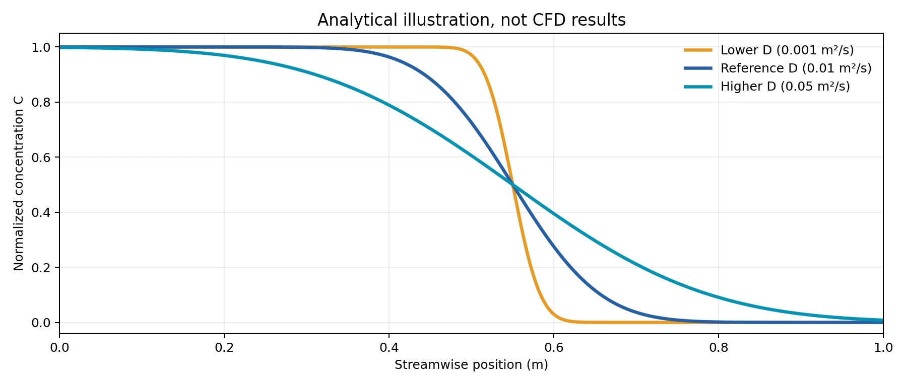
Figure 3 — Illustrative analytical front profiles for different parameters; these are not OpenFOAM outputs.
Export A_reference.csv, B_low_diffusivity.csv and C_high_diffusivity.csv from ParaView’s Plot Over Line using File > Save Data with identical time/line settings.
Deep dive · Additional script: front_metrics.py (position, thickness, apparent diffusivity)
It turns a profile into three numbers comparable across cases: front position x50, 10–90 % thickness and equivalent one-dimensional diffusivity Dapp = (w10–90/3.6252)²/t. Dapp lumps physical diffusion, shear dispersion, numerical diffusion and velocity non-uniformity: it is not a measurement of D, but it shows how much apparent diffusion depends on numerics and flow.
python3 front_metrics.py exports/A_reference.csv exports/B_low_diffusivity.csv exports/C_high_diffusivity.csv \
       --time 0.02 --output front_t002.csv
python3 front_metrics.py exports/D_half_inlet.csv --cref 0.5 --time 0.02 --output front_half_t002.csv
Checks performed: on the three synthetic CSVs of the package (illustrative erfc fronts centred at 0.52 m) with --time 0.2 the script returns Dapp = 0.0100, 0.00106 and 0.0500 m²/s, i.e. the nominal values (the deviation for B comes from the 10 mm sampling step, coarse compared with a 53 mm front); on the Ogata–Banks analytical solution with U = 5 m/s, D = 0.01 m²/s, t = 0.02 s it returns 0.0097 m²/s.
#!/usr/bin/env python3
# SPDX-License-Identifier: GPL-3.0-or-later
"""Front metrics from ParaView Plot Over Line exports (columns arc_length, C).

For every CSV given on the command line the script finds, scanning from the
start of the line, the first positions where C falls below 0.9, 0.5 and 0.1
times the reference value (--cref, default 1; use 0.5 for D_half_inlet),
with linear interpolation between samples. It reports:
  x50      front position (C = 0.5 Cref)            [m]
  w10_90   front thickness x10 - x90                 [m]
  D_app    equivalent 1D diffusivity (w10_90 / 3.6252)^2 / t_front   [m2/s]
For an erfc front of a 1D advection-diffusion problem w10_90 = 2 erfinv(0.8)
* 2 sqrt(D t) = 3.6252 sqrt(D t). D_app therefore lumps physical diffusion,
shear (Taylor) dispersion, numerical diffusion and non-uniform velocity: it
is a diagnostic to COMPARE cases on the same line, mesh and time, not a
measurement of D. t_front is the time the front has been travelling
(--time, the physical time of the export, by default).
A NEW CSV is written; existing files are never overwritten.
"""
import argparse
import csv
import math
from pathlib import Path
import sys

K = 2 * 2 * 0.9061938024368232      # 2 * erfinv(0.8) * 2


def read(path):
    with path.open(newline='', encoding='utf-8-sig') as f:
        r = csv.DictReader(f)
        keys = r.fieldnames or []
        xk = next((k for k in keys if k.strip().lower() in ('arc_length', 'arc length')), None)
        ck = next((k for k in keys if k.strip() == 'C'), None)
        if not xk or not ck:
            raise ValueError(f'{path.name}: columns arc_length and C are required, found {keys}')
        rows = []
        for row in r:
            try:
                x, c = float(row[xk]), float(row[ck])
            except (TypeError, ValueError):
                continue
            if math.isfinite(x) and math.isfinite(c):
                rows.append((x, c))
    rows.sort()
    if len(rows) < 3:
        raise ValueError(f'{path.name}: fewer than 3 valid samples')
    return rows


def crossing(rows, level):
    """First x where C goes from >= level to < level (linear interpolation)."""
    for (x0, c0), (x1, c1) in zip(rows, rows[1:]):
        if c0 >= level > c1:
            return x0 + (level - c0) * (x1 - x0) / (c1 - c0)
    return None


def main():
    p = argparse.ArgumentParser(description=__doc__, formatter_class=argparse.RawDescriptionHelpFormatter)
    p.add_argument('csv', type=Path, nargs='+')
    p.add_argument('--time', type=float, help='front travel time t_front [s] (needed for D_app)')
    p.add_argument('--cref', type=float, default=1.0, help='inlet value of C (0.5 for D_half_inlet)')
    p.add_argument('--output', type=Path, required=True, help='NEW csv file')
    a = p.parse_args()
    if a.output.exists():
        p.error('Output exists; refusing to overwrite it')
    out = []
    for f in a.csv:
        rows = read(f)
        cmin, cmax = min(c for _, c in rows), max(c for _, c in rows)
        x90, x50, x10 = (crossing(rows, lv * a.cref) for lv in (0.9, 0.5, 0.1))
        w = (x10 - x90) if (x10 is not None and x90 is not None) else None
        dapp = (w / K) ** 2 / a.time if (w is not None and a.time) else None
        out.append(dict(file=f.name, n=len(rows), C_min=f'{cmin:.6g}', C_max=f'{cmax:.6g}',
                        overshoot=f'{max(0.0, cmax - a.cref):.3g}', undershoot=f'{max(0.0, -cmin):.3g}',
                        x90_m='' if x90 is None else f'{x90:.6g}', x50_m='' if x50 is None else f'{x50:.6g}',
                        x10_m='' if x10 is None else f'{x10:.6g}', w10_90_m='' if w is None else f'{w:.6g}',
                        D_app_m2_s='' if dapp is None else f'{dapp:.4g}'))
        msg = f'{f.name}: C in [{cmin:.4g}, {cmax:.4g}]'
        msg += f', x50 = {x50:.4g} m' if x50 is not None else ', no 0.5 crossing (front outside the line?)'
        if w is not None:
            msg += f', w10-90 = {w * 1000:.3g} mm'
        if dapp is not None:
            msg += f', D_app = {dapp:.3g} m2/s'
        print(msg)
    with a.output.open('x', newline='', encoding='utf-8') as f:
        wr = csv.DictWriter(f, fieldnames=list(out[0]))
        wr.writeheader()
        wr.writerows(out)
    print('Written', a.output, '- D_app is an equivalent 1D value, not the molecular D.')


if __name__ == '__main__':
    try:
        main()
    except (OSError, ValueError) as exc:
        sys.exit(f'ERROR: {exc}')
Deep dive · Analytical reference solution: Ogata and Banks (1961)
For a semi-infinite domain with uniform velocity U, constant D, initial C = 0 and C = C0 at the inlet:
C/C0 = 1/2 [ erfc((x - U t)/(2 sqrt(D t))) + exp(U x/D) erfc((x + U t)/(2 sqrt(D t))) ]This is the classical solution of Ogata and Banks, USGS Professional Paper 411-A, 1961 (doi:10.3133/pp411A). The following script writes it to a CSV with the same columns as ParaView, so it can be used with compare_profiles.py and front_metrics.py. The second term is computed in a stable form even for very large U x/D; the equation residual, checked with finite differences, is of the order of 6·10⁻⁷. For a code verification (not physics) a 1D channel with uniform velocity can be built and the profiles compared directly: this is Guide 4 verification applied to transport.
python3 ogata_banks.py --U 5 --D 0.01 --t 0.02 --L 0.3 --n 1001 --output analytic_D001_t002.csv#!/usr/bin/env python3
# SPDX-License-Identifier: GPL-3.0-or-later
"""Analytic 1D advection-diffusion front (Ogata & Banks, 1961) for verification.
Semi-infinite domain x >= 0, uniform velocity U, constant D, C(x,0) = 0,
C(0,t) = C0:
C/C0 = 1/2 [ erfc((x - U t)/(2 sqrt(D t))) + exp(U x / D) erfc((x + U t)/(2 sqrt(D t))) ]
The second term is evaluated in a numerically safe form for large U x / D.
Writes a NEW CSV with columns arc_length and C, directly comparable with
compare_profiles.py and with a ParaView Plot Over Line export of a 1D channel.
"""
import argparse
import csv
import math
from pathlib import Path
def front(x, t, U, D, C0=1.0):
if t <= 0:
return 0.0
s = 2.0 * math.sqrt(D * t)
a = math.erfc((x - U * t) / s)
z = (x + U * t) / s
# exp(Ux/D) * erfc(z) = exp(Ux/D - z^2) * erfcx(z); use asymptotics when z is large
if z < 25:
b = math.exp(U * x / D) * math.erfc(z) if U * x / D < 700 else 0.0
else:
b = math.exp(U * x / D - z * z) / (z * math.sqrt(math.pi)) * (1 - 1 / (2 * z * z))
return 0.5 * C0 * (a + b)
def main():
p = argparse.ArgumentParser(description=__doc__)
p.add_argument('--U', type=float, required=True, help='velocity [m/s]')
p.add_argument('--D', type=float, required=True, help='diffusivity [m2/s]')
p.add_argument('--t', type=float, required=True, help='time [s]')
p.add_argument('--L', type=float, required=True, help='profile length [m]')
p.add_argument('--n', type=int, default=201, help='number of samples')
p.add_argument('--C0', type=float, default=1.0)
p.add_argument('--output', type=Path, required=True, help='NEW csv file')
a = p.parse_args()
if a.output.exists():
p.error('Output exists; refusing to overwrite it')
if min(a.D, a.t, a.L) <= 0 or a.n < 3:
p.error('D, t, L must be > 0 and n >= 3')
with a.output.open('x', newline='', encoding='utf-8') as f:
w = csv.writer(f)
w.writerow(['arc_length', 'C'])
for i in range(a.n):
x = a.L * i / (a.n - 1)
w.writerow([f'{x:.8g}', f'{front(x, a.t, a.U, a.D, a.C0):.8g}'])
width = 2 * math.sqrt(a.D * a.t)
print(f'Front centre U t = {a.U * a.t:.6g} m, diffusive width 2 sqrt(D t) = {width:.6g} m, Pe_L = {a.U * a.L / a.D:.4g}')
print('Written', a.output)
if __name__ == '__main__':
main()Deep dive · The recirculation bubble: where D matters longest
In a frozen mean field the streamlines of the bubble behind the step are closed: the tracer enters the bubble only across the dividing streamline, i.e. by diffusion. An order of magnitude of the filling time is h²/D with h ≈ 25 mm: about 0.65 s for D = 0.001, 0.065 s for D = 0.01, 0.013 s for D = 0.05. In case B, therefore, the bubble does not fill within 0.2 s, while in case C it is full after a few hundredths of a second. A second sampling line in the bubble (box in section 4) and the volIntegrate(C) inventory make this effect visible, the strongest in the whole campaign.
In the real flow turbulent fluctuations exchange fluid between bubble and jet: in a RANS model this exchange is represented precisely by νt/Sct, which justifies the E_turbulent case proposed in section 2.
Practical tip · Convergence study: beware, the mesh cannot be refined on its own
The 0/U, 0/phi and 0/nut fields are lists of 12 225 cells and 24 170 faces: they are only valid for the original mesh. For a mesh study the flow must be recomputed on the refined mesh (for example with the steady incompressibleFluid/pitzDailySteady tutorial and a blockMeshDict with twice the cells in each direction) and only then scalarTransport run with solver functions. Interpolating phi from one mesh to another would produce a non-conservative flux and a corrupted balance. The time-step study, on the other hand, is immediate (section 3).
10. Exercise 3 — A linearity check
Compare A_reference and D_half_inlet with identical D. For this linear source-free model and consistent initial and boundary conditions, the tracer field should be approximately half the reference at the same instant:
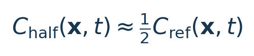
Small discrepancies may arise from solver tolerance and numerical errors. Large discrepancies require checks of mesh, U, phi, schemes and sampling times.
Deep dive · Why linearity holds (and when it stops holding)
With Gauss linearUpwind grad(C) and Gauss linear gradient the discrete operator is linear in C: the algebraic system of each step is M Cn+1 = b(Cn, Cin) with M independent of C. Multiplying the inlet condition and the (zero) initial condition by λ multiplies the discrete solution exactly by λ; the only deviations come from the solver tolerance (10⁻⁶ absolute, hence relatively twice as large for the halved case).
- TVD schemes (
limitedLinear,vanLeer) depend on the ratio of successive gradients, which does not change when C is multiplied by λ > 0: proportionality stays exact, although superposition of two different solutions no longer holds. - The “01” variants and MULES compare C with fixed bounds (0 and 1): proportionality is no longer guaranteed and the test fails by construction, not because of an error.
- A case with different D, different mesh or different
phiis not comparable: this is why the test usesA_referenceandD_half_inlet, identical except for the inlet value.
Deep dive · Additional script: linearity_check.py
It quantifies the deviation |Chalf − λ Cref| on the ParaView profiles or, better, on the .dat files of the function objects (inventory, outlet concentration), which cover all time steps and do not depend on ParaView interpolation. On the synthetic CSVs of the package it returns a deviation of 5·10⁻⁸ and λ = 0.50000000.
python3 linearity_check.py profiles exports/A_reference.csv exports/D_half_inlet.csv
python3 linearity_check.py dat \
  A_reference/postProcessing/volIntegrate\(C\)/0/volFieldValue.dat \
  D_half_inlet/postProcessing/volIntegrate\(C\)/0/volFieldValue.dat
The folder name in postProcessing is the name of the function object: check with ls postProcessing (parentheses must be escaped in the shell).
#!/usr/bin/env python3
# SPDX-License-Identifier: GPL-3.0-or-later
"""Quantitative linearity test between A_reference and D_half_inlet.

Two modes, both read-only:
  profiles: two ParaView Plot Over Line CSVs (arc_length, C) at the SAME time
            and on the SAME line;
  dat:      two .dat files of the same function object (for example
            volIntegrate(C) or CbulkOutlet) written by the two cases.
The expected relation is C_half = lambda * C_ref with lambda = 0.5. The script
prints the maximum absolute deviation |C_half - lambda C_ref|, the same value
divided by max|C_ref| and the best-fit lambda (least squares). With an
unlimited linear scheme (linearUpwind) the deviation should be of the order of
the solver tolerance; TVD limiters keep the scaling exactly in exact
arithmetic; MULES or "01" limiters with fixed bounds do not.
"""
import argparse
import csv
import math
from pathlib import Path
import sys


def read_csv(path):
    with path.open(newline='', encoding='utf-8-sig') as f:
        r = csv.DictReader(f)
        keys = r.fieldnames or []
        xk = next((k for k in keys if k.strip().lower() in ('arc_length', 'arc length')), None)
        ck = next((k for k in keys if k.strip() == 'C'), None)
        if not xk or not ck:
            raise ValueError(f'{path.name}: columns arc_length and C are required')
        rows = []
        for row in r:
            try:
                x, c = float(row[xk]), float(row[ck])
            except (TypeError, ValueError):
                continue
            if math.isfinite(x) and math.isfinite(c):
                rows.append((x, c))
    return sorted(rows)


def read_dat(path, column):
    out = []
    with open(path, encoding='utf-8') as f:
        for line in f:
            s = line.strip()
            if s and not s.startswith('#'):
                p = s.replace('(', ' ').replace(')', ' ').split()
                out.append((float(p[0]), float(p[column - 1])))
    return sorted(out)


def main():
    p = argparse.ArgumentParser(description=__doc__, formatter_class=argparse.RawDescriptionHelpFormatter)
    p.add_argument('mode', choices=('profiles', 'dat'))
    p.add_argument('reference', type=Path)
    p.add_argument('half', type=Path)
    p.add_argument('--lam', type=float, default=0.5)
    p.add_argument('--column', type=int, default=2, help='column of the .dat files')
    a = p.parse_args()
    if a.mode == 'profiles':
        ref, half = read_csv(a.reference), read_csv(a.half)
    else:
        ref, half = read_dat(a.reference, a.column), read_dat(a.half, a.column)
    hmap = dict(half)
    pairs = [(c, hmap[x]) for x, c in ref if x in hmap]
    if len(pairs) < 3:
        raise ValueError('fewer than 3 common abscissae/times: use the same line, resolution and times')
    dev = max(abs(h - a.lam * c) for c, h in pairs)
    scale = max(abs(c) for c, _ in pairs) or 1.0
    den = sum(c * c for c, _ in pairs)
    lam_fit = sum(c * h for c, h in pairs) / den if den else float('nan')
    print(f'{len(pairs)} common points; max |C_half - {a.lam:g} C_ref| = {dev:.3e} ({dev / scale:.3e} of max|C_ref|)')
    print(f'best-fit lambda = {lam_fit:.8f}')


if __name__ == '__main__':
    try:
        main()
    except (OSError, ValueError, IndexError) as exc:
        sys.exit(f'ERROR: {exc}')
11. Conservation check and physical meaning
With outward-pointing surface normal n and no sources, the integral balance is:

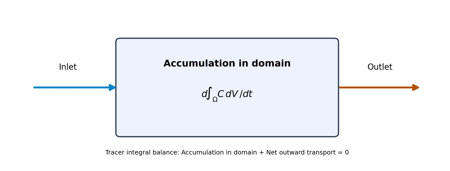
Figure 4 — Conceptual balance: accumulation plus net outward transport equals zero.
Data sampled along a line cannot close this volume balance. A quantitative check requires integrated volume inventory, advective and diffusive fluxes through all boundary surfaces, and time resolution. For basic qualitative diagnostics, record scalar minima/maxima, front position, apparent front width, and any oscillation or overshoot.
Optional refresher — Numerical diffusion. A discrete advection scheme may smear a steep front even at small physical D. Repeat studies with refined meshes and reduced time steps as explained in Guide 4; a visually pleasing curve is not evidence of convergence.
Deep dive · The discrete balance with function objects (tracer_balance.py script)
With the monitoring file of section 5 the inventory I(t) = ∫C dV and the advective inlet Σφ C (negative) and outlet (positive) flows are available at every step. The advective balance is
dI/dt + sum_outlet(phi C) + sum_inlet(phi C) = diffusive inflow at the inlet + numerical errorAt the outlet and walls the zeroGradient condition cancels the diffusive flux; at the inlet fixedValue instead leaves a diffusive flux D (Cin − CP)/δ, large in the first steps and zero once the adjacent cell reaches Cin. The script computes dI/dt with central differences, interpolates the flows at the same times and writes the absolute residual and the residual relative to the inflow. On a consistent synthetic series the residual is of the order of 10⁻¹¹ m³/s (5·10⁻⁷ of the inflow).
cd "$HOME/cases/guide12_species_01/A_reference/postProcessing"
python3 tracer_balance.py --inventory "volIntegrate(C)/0/volFieldValue.dat" \
  --inlet CflowInlet/0/surfaceFieldValue.dat --outlet CflowOutlet/0/surfaceFieldValue.dat \
  --every 10 --output ../tracer_balance_A.csv
#!/usr/bin/env python3
# SPDX-License-Identifier: GPL-3.0-or-later
"""Tracer inventory balance from OpenFOAM function-object .dat files.
Inputs (written by the functions of Guide 12, one value per time step):
--inventory volFieldValue volIntegrate(C) file -> I(t) [m3]
--inlet surfaceFieldValue sum(phi*C) on the inlet -> negative [m3/s]
--outlet surfaceFieldValue sum(phi*C) on the outlet -> positive [m3/s]
Advective balance: dI/dt + (sum_outlet + sum_inlet) = diffusive inflow + error.
With zeroGradient at outlet and walls, the remaining term is the diffusive
flux through the fixedValue inlet plus the numerical error. A NEW CSV is
written; existing files are never overwritten.
"""
import argparse
import csv
from pathlib import Path
import sys
def read(path, column):
t, v = [], []
with open(path, encoding='utf-8') as f:
for n, line in enumerate(f, 1):
s = line.strip()
if not s or s.startswith('#'):
continue
parts = s.replace('(', ' ').replace(')', ' ').split()
try:
t.append(float(parts[0]))
v.append(float(parts[column - 1]))
except (IndexError, ValueError) as exc:
raise ValueError(f'{path}:{n}: cannot read column {column}') from exc
if len(t) < 3:
raise ValueError(f'{path}: at least three records are required')
pairs = sorted(dict(zip(t, v)).items())
return [x for x, _ in pairs], [y for _, y in pairs]
def at(ts, vs, x):
if x <= ts[0]:
return vs[0]
if x >= ts[-1]:
return vs[-1]
for i in range(1, len(ts)):
if x <= ts[i]:
w = (x - ts[i - 1]) / (ts[i] - ts[i - 1])
return vs[i - 1] + w * (vs[i] - vs[i - 1])
return vs[-1]
def main():
p = argparse.ArgumentParser(description=__doc__, formatter_class=argparse.RawDescriptionHelpFormatter)
p.add_argument('--inventory', type=Path, required=True)
p.add_argument('--inlet', type=Path, required=True)
p.add_argument('--outlet', type=Path, required=True)
p.add_argument('--column', type=int, default=2)
p.add_argument('--every', type=int, default=10, help='one output row every N records')
p.add_argument('--output', type=Path, required=True)
a = p.parse_args()
if a.output.exists():
p.error('Output exists; refusing to overwrite it')
ti, vi = read(a.inventory, a.column)
tin, vin = read(a.inlet, a.column)
tout, vout = read(a.outlet, a.column)
rows = []
for k in range(1, len(ti) - 1, max(1, a.every)):
t = ti[k]
didt = (vi[k + 1] - vi[k - 1]) / (ti[k + 1] - ti[k - 1])
adv_in = -at(tin, vin, t)
adv_out = at(tout, vout, t)
residual = didt - adv_in + adv_out
rows.append(dict(time_s=f'{t:.6g}', inventory_m3=f'{vi[k]:.6g}', dI_dt_m3_s=f'{didt:.6g}',
advective_in_m3_s=f'{adv_in:.6g}', advective_out_m3_s=f'{adv_out:.6g}',
residual_m3_s=f'{residual:.6g}',
residual_over_inflow=f'{residual / adv_in:.4g}' if adv_in else 'nan'))
with a.output.open('x', newline='', encoding='utf-8') as f:
w = csv.DictWriter(f, fieldnames=list(rows[0]))
w.writeheader()
w.writerows(rows)
last = rows[-1]
print(f'{len(rows)} rows written to {a.output}')
print(f"t = {last['time_s']} s: dI/dt = {last['dI_dt_m3_s']}, in = {last['advective_in_m3_s']}, "
f"out = {last['advective_out_m3_s']}, residual = {last['residual_m3_s']} ({last['residual_over_inflow']} of inflow)")
print('The residual contains the diffusive inflow at the inlet and the numerical error.')
if __name__ == '__main__':
try:
main()
except (OSError, ValueError) as exc:
sys.exit(f'ERROR: {exc}')Deep dive · Three global checks that need no script
- First instant: dI/dt ≈ Q·Cin = 2.54·10⁻⁴ m³/s (Cin = 1) and 1.27·10⁻⁴ m³/s for
D_half_inlet, until the front reaches the outlet. - Long time: I(t) → V = 1.452·10⁻⁵ m³ and inlet and outlet flows become equal and opposite.
- Bounds:
cellMin(C)≥ 0 andcellMax(C)≤ Cin at every step (maximum principle); report the worst value and its time.
The time integral of (1 − I(t)/V) measures how long the domain takes to fill: it is related to the mean residence time (box in section 12).
12. Processing CSVs on Windows
Export Plot Over Line data with arc_length and C columns, and save locally (or transfer using FileZilla). With Python 3 on Windows:
python compare_profiles.py exports output_guide12_01The standard-library-only tool produces profile_summary.csv, pointwise_difference.csv, and profile_comparison.svg; it refuses to overwrite an existing output folder. Line-sampled averages and standard deviations are not mixing efficiency, flow-weighted outlet means, or mass conservation checks.
For a physically meaningful outlet mixing metric, prefer a flow-weighted variance relative to a specified mean and, where relevant, species mass flow. Do not confuse spatial heterogeneity with time-averaged variation.
Deep dive · Package script: compare_profiles.py
It uses only the standard library: it reads CSVs with arc_length and C columns (tolerates Excel’s BOM and discards non-numeric or non-finite rows), requires strictly increasing abscissae, and writes per-case statistics, an SVG plot and pointwise differences with respect to A_reference where the supports overlap. Tested with the four synthetic CSVs: three files produced, 303 difference rows.
An instructive example of the guide’s warning: on the synthetic CSVs A, B and C the sample mean is 0.520 in all three cases, because the fronts share the same centre and are symmetric; only the standard deviation changes (0.463, 0.488, 0.413). The unweighted mean along a line therefore cannot tell a better-mixed case from a less-mixed one.
#!/usr/bin/env python3
# SPDX-License-Identifier: GPL-3.0-or-later
"""Compare ParaView Plot Over Line CSV exports using only the Python standard library.

Run: python compare_profiles.py exports_folder output_folder
Expected: A_reference.csv, B_low_diffusivity.csv,
          C_high_diffusivity.csv and optionally D_half_inlet.csv.
Select the same time and the same sampling line in every case.
"""
import csv
import html
import math
import sys
from pathlib import Path
from statistics import fmean, pstdev

CASES = ['A_reference', 'B_low_diffusivity', 'C_high_diffusivity', 'D_half_inlet']
COLORS = ['#2563eb', '#d97706', '#0891b2', '#7c3aed']


def read_csv(path):
    with path.open('r', newline='', encoding='utf-8-sig') as f:
        reader = csv.DictReader(f)
        if not reader.fieldnames:
            raise ValueError(f'Empty file: {path}')
        keys = reader.fieldnames
        x = next((k for k in keys if k.strip().lower() in ('arc_length', 'arc length')), None)
        c = next((k for k in keys if k.strip() == 'C'), None)
        if not x or not c:
            raise ValueError(f'{path.name}: expected arc_length and C columns; found {keys}')
        rows = []
        for r in reader:
            try:
                xv, cv = float(r[x]), float(r[c])
            except (TypeError, ValueError):
                continue
            if math.isfinite(xv) and math.isfinite(cv):
                rows.append((xv, cv))
    rows.sort()
    # Reject duplicated coordinates rather than silently altering profiles.
    if len(rows) < 3 or any(rows[i][0] <= rows[i-1][0] for i in range(1, len(rows))):
        raise ValueError(f'{path.name}: require at least 3 strictly increasing x values')
    return rows


def interp(rows, x):
    if x < rows[0][0] or x > rows[-1][0]:
        return None
    lo, hi = 0, len(rows) - 1
    while hi - lo > 1:
        k = (lo + hi) // 2
        if rows[k][0] < x:
            lo = k
        else:
            hi = k
    a, b = rows[lo], rows[hi]
    return a[1] + (b[1] - a[1]) * (x - a[0]) / (b[0] - a[0])


def svg_plot(data):
    allpts = [pt for rows in data.values() for pt in rows]
    xmin = min(p[0] for p in allpts)
    xmax = max(p[0] for p in allpts)
    ymin = min(0, min(p[1] for p in allpts))
    ymax = max(1, max(p[1] for p in allpts))
    if xmax <= xmin: xmax = xmin + 1
    if ymax <= ymin: ymax = ymin + 1
    w, h = 1000, 570
    X = lambda a: 85 + 855 * (a - xmin) / (xmax - xmin)
    Y = lambda a: 485 - 395 * (a - ymin) / (ymax - ymin)
    parts = [f'<svg xmlns="http://www.w3.org/2000/svg" viewBox="0 0 {w} {h}" role="img" aria-label="Tracer profiles">',
             '<rect width="100%" height="100%" fill="white"/>',
             '<path d="M85 90 V485 H940" fill="none" stroke="#334155" stroke-width="2"/>']
    for j in range(5):
        val = ymin + (ymax-ymin)*j/4
        yy = Y(val)
        parts.append(f'<path d="M85 {yy:.1f} H940" stroke="#e2e8f0"/>')
        parts.append(f'<text x="70" y="{yy+5:.1f}" font-size="15" text-anchor="end">{val:.2f}</text>')
    for j in range(5):
        val=xmin+(xmax-xmin)*j/4
        xx=X(val)
        parts.append(f'<text x="{xx:.1f}" y="510" font-size="15" text-anchor="middle">{val:.3g}</text>')
    parts.extend(['<text x="515" y="550" text-anchor="middle" font-size="18">arc_length (m)</text>',
                  '<text x="23" y="270" transform="rotate(-90 23 270)" text-anchor="middle" font-size="18">C (dimensionless)</text>'])
    for (name,rows),color in zip(data.items(), COLORS):
        points=' '.join(f'{X(x):.1f},{Y(y):.1f}' for x,y in rows)
        parts.append(f'<polyline points="{points}" fill="none" stroke="{color}" stroke-width="3"/>')
    for idx,(name,rows) in enumerate(data.items()):
        y=30+idx*22
        parts.append(f'<line x1="680" y1="{y}" x2="710" y2="{y}" stroke="{COLORS[idx]}" stroke-width="4"/>')
        parts.append(f'<text x="715" y="{y+5}" font-size="16">{html.escape(name)}</text>')
    parts.append('</svg>')
    return '\n'.join(parts)


def main():
    if len(sys.argv) != 3:
        raise SystemExit('Usage: python compare_profiles.py exports_folder output_folder')
    inp, out = Path(sys.argv[1]), Path(sys.argv[2])
    if out.exists():
        raise SystemExit(f'Output directory already exists (no overwrite): {out}')
    data={}
    for name in CASES:
        file=inp/(name+'.csv')
        if file.is_file(): data[name]=read_csv(file)
    if not {'A_reference','B_low_diffusivity','C_high_diffusivity'}.issubset(data):
        raise SystemExit('Expected A_reference, B_low_diffusivity and C_high_diffusivity CSVs')
    out.mkdir(parents=True)
    with (out/'profile_summary.csv').open('w',newline='',encoding='utf-8') as f:
        writer=csv.writer(f)
        writer.writerow(['case','n_samples','min_C','max_C','sample_mean_C','sample_std_C','note'])
        for name,rows in data.items():
            values=[p[1] for p in rows]
            writer.writerow([name,len(rows),min(values),max(values),fmean(values),pstdev(values),
                             'Unweighted sample-line stats; NOT mixing efficiency or mass balance'])
    (out/'profile_comparison.svg').write_text(svg_plot(data),encoding='utf-8')
    # Pointwise comparison where supports overlap (not an integral conservation test).
    baseline=data['A_reference']
    with (out/'pointwise_difference.csv').open('w',newline='',encoding='utf-8') as f:
        writer=csv.writer(f)
        writer.writerow(['case','arc_length_m','C_case_minus_reference'])
        for name,rows in data.items():
            if name=='A_reference':continue
            for x,y in baseline:
                v=interp(rows,x)
                if v is not None: writer.writerow([name,x,v-y])
    print(f'Created outputs under: {out}')
    print('Not a validation of mass conservation or mixing efficiency.')

if __name__=='__main__':
    main()
Deep dive · Flow-weighted mixing indices: mean, variance, intensity of segregation
The cup-mixing concentration on a section is c̄ = Σφ C/Σφ, already computed by CbulkOutlet. For the flow-weighted variance ⟨C²⟩φ is also needed: compute C² with magSqr and take its weighted average:
// add to system/functions (before the run)
#includeFunc magSqr(C, executeControl=timeStep, writeControl=writeTime)

C2bulkOutlet
{
    type            surfaceFieldValue;
    libs            ("libfieldFunctionObjects.so");
    writeControl    timeStep;
    writeInterval   1;
    writeFields     false;
    patch           outlet;
    operation       average;
    weightField     phi;
    fields          (magSqr(C));
}
sigma^2 = <C^2>_phi - c_bar^2 flow-weighted variance
CoV = sigma / c_bar coefficient of variation
I_s = sigma^2 / (c_bar (1 - c_bar)) intensity of segregation (Danckwerts)The intensity of segregation is 1 for fully segregated streams and 0 for a perfectly mixed section (doi:10.1007/BF03184936, Danckwerts 1952). In this single-inlet case the value is meaningful only while the front passes; it becomes the main index in a two-inlet mixer (for example C = 1 in one and C = 0 in the other). The two functions must be declared in the order shown, because magSqr(C) must exist when the average is computed.
Deep dive · Residence time distribution from the tracer (rtd_moments.py script)
With C = 0 initially and a step Cin at the inlet, F(t) = c̄out(t)/Cin is Danckwerts’ F curve (step response) and E(t) = dF/dt the residence time distribution (doi:10.1016/0009-2509(53)80001-1, Danckwerts 1953). The mean time τm = ∫(1 − F) dt must equal the space time V/Q = 57.1 ms for a closed vessel without diffusion through inlet and outlet (doi:10.1021/ie071635a, Nauman 2008): it is an independent check of both conservation and the flow field.
Mind the tail: with endTime 0.2 (3.5 τ) the F curve does not reach 1, especially because of the recirculation bubble. On a synthetic perfectly-mixed-reactor curve with τ = 57.1 ms the script returns τm = 55.4 ms when truncated at 0.2 s (F = 0.970) and 57.1 ms when extended to 2 s. For a reliable RTD use a copy with endTime 1 or more: the field is frozen and the cost is minimal.
python3 rtd_moments.py A_reference/postProcessing/CbulkOutlet/0/surfaceFieldValue.dat \
       --volume 1.4516e-5 --flow 2.54e-4 --output rtd_A.csv
#!/usr/bin/env python3
# SPDX-License-Identifier: GPL-3.0-or-later
"""Step-response (F-curve) analysis of the flow-weighted outlet tracer.
Input: the .dat file of the CbulkOutlet function (surfaceFieldValue,
operation average, weightField phi) of a case with C(inlet) = Cin and C = 0
initially. F(t) = Cbulk(t)/Cin is the Danckwerts F-curve (step response) and
E(t) = dF/dt the residence time distribution. The script prints
t10, t50, t90 times at which F reaches 0.1, 0.5, 0.9 [s]
tau_m = int (1-F) dt mean residence time (truncated at the last record)
sigma2 = 2 int t (1-F) dt - tau_m^2 variance of E (truncated)
F_end value of F at the last record (tail not yet seen if < 1)
and compares tau_m with the space time V/Q if --volume and --flow are given.
For a closed vessel without diffusion through inlet and outlet
tau_m = V/Q (Danckwerts 1953; Nauman 2008). A NEW CSV with t, F, E is written.
"""
import argparse
import csv
from pathlib import Path
import sys
def read(path, column):
t, v = [], []
with open(path, encoding='utf-8') as f:
for n, line in enumerate(f, 1):
s = line.strip()
if not s or s.startswith('#'):
continue
parts = s.replace('(', ' ').replace(')', ' ').split()
try:
t.append(float(parts[0]))
v.append(float(parts[column - 1]))
except (IndexError, ValueError) as exc:
raise ValueError(f'{path}:{n}: cannot read column {column}') from exc
pairs = sorted(dict(zip(t, v)).items())
if len(pairs) < 3:
raise ValueError(f'{path}: at least three records are required')
return [a for a, _ in pairs], [b for _, b in pairs]
def first_time(t, F, level):
for i in range(1, len(t)):
if F[i - 1] < level <= F[i]:
return t[i - 1] + (level - F[i - 1]) * (t[i] - t[i - 1]) / (F[i] - F[i - 1])
return None
def main():
p = argparse.ArgumentParser(description=__doc__, formatter_class=argparse.RawDescriptionHelpFormatter)
p.add_argument('dat', type=Path, help='CbulkOutlet .dat file')
p.add_argument('--column', type=int, default=2)
p.add_argument('--cin', type=float, default=1.0, help='inlet value of C')
p.add_argument('--volume', type=float, help='domain volume V [m3] (checkMesh)')
p.add_argument('--flow', type=float, help='volumetric flow Q [m3/s]')
p.add_argument('--output', type=Path, required=True, help='NEW csv file')
a = p.parse_args()
if a.output.exists():
p.error('Output exists; refusing to overwrite it')
t, c = read(a.dat, a.column)
if t[0] > 0: # the step starts at t = 0 with F = 0
t, c = [0.0] + t, [0.0] + c
F = [x / a.cin for x in c]
tau = sum((t[i] - t[i - 1]) * (2 - F[i] - F[i - 1]) / 2 for i in range(1, len(t)))
m1 = sum((t[i] - t[i - 1]) * (t[i] * (1 - F[i]) + t[i - 1] * (1 - F[i - 1])) / 2 for i in range(1, len(t)))
sigma2 = 2 * m1 - tau ** 2
E = [0.0] + [(F[i] - F[i - 1]) / (t[i] - t[i - 1]) for i in range(1, len(t))]
with a.output.open('x', newline='', encoding='utf-8') as f:
w = csv.writer(f)
w.writerow(['time_s', 'F', 'E_1_s'])
for row in zip(t, F, E):
w.writerow([f'{row[0]:.8g}', f'{row[1]:.8g}', f'{row[2]:.8g}'])
for lv in (0.1, 0.5, 0.9):
x = first_time(t, F, lv)
print(f't{int(lv * 100)} = ' + (f'{x * 1000:.3f} ms' if x is not None else 'not reached'))
print(f'F at the last record (t = {t[-1]:g} s) = {F[-1]:.6f}' + ('' if F[-1] > 0.999 else ' -> tail truncated: tau_m is a lower bound'))
print(f'tau_m = int(1-F)dt = {tau * 1000:.3f} ms, sigma = {max(sigma2, 0) ** 0.5 * 1000:.3f} ms')
if a.volume and a.flow:
st = a.volume / a.flow
print(f'space time V/Q = {st * 1000:.3f} ms, tau_m/(V/Q) = {tau / st:.4f}')
print('Written', a.output)
if __name__ == '__main__':
try:
main()
except (OSError, ValueError) as exc:
sys.exit(f'ERROR: {exc}')Deep dive · Local mean age with the age function object
OpenFOAM 14 also solves the steady mean-age equation ∇·(φ a) = 1 (age.H), with automatically generated conditions (zeroGradient on walls, inletOutlet elsewhere) and diffusion off by default. The transport formulation of local age is discussed by doi:10.1016/j.ces.2003.10.013 (Ghirelli and Leckner 2004). The flow-weighted mean of the age at the outlet must equal V/Q:
// in a separate copy: schemes and solver of C are reused
#includeFunc age(schemesField=C, solverField=C)

ageBulkOutlet
{
    type            surfaceFieldValue;
    libs            ("libfieldFunctionObjects.so");
    writeControl    writeTime;
    writeFields     false;
    patch           outlet;
    operation       average;
    weightField     phi;
    fields          (age);
}
The age field directly shows stagnant regions (the bubble has ages much larger than τ). With the linearUpwind scheme a few corrections are needed (nCorrectors 5 by default); with upwind one is enough, as stated in the configuration description.
Practical tip · Python on Windows: commands and folders
py -3 --version
py -3 compare_profiles.py exports output_guide12_01
py -3 front_metrics.py exports\A_reference.csv --time 0.02 --output output_guide12_01_front.csv
The py launcher is installed with Python for Windows. Output folders must not exist: use a progressive suffix (_01, _02…) instead of deleting earlier results.
13. Chemical-engineering limits and next steps
Passive-tracer transport is useful for a sufficiently dilute scalar that does not modify flow properties. It does not automatically model multicomponent nonideal diffusion, variable-density mixtures, large viscosity changes, chemical reactions, emulsions, immiscible-phase interfaces, oil/water partition, or interphase mass-transfer resistance. Such systems require additional governing equations and physical closure models, and often multiphase CFD.
This exercise builds foundations for mixers, microreactors and extraction columns. Guide 13 moves to multiphase interfaces; later guides address reaction/transport coupling.
Deep dive · Beyond the passive tracer: what OpenFOAM 14 offers
| Need | Tool in OpenFOAM 14 |
|---|---|
| tracer in one phase of a two-phase flow (VoF) | phaseScalarTransport, tutorial incompressibleVoF/damBreakLaminar/damBreakTracer (Guide 13) |
| species affecting density or properties | fluid module (multicomponent) with mass fractions Yi |
| Fickian species diffusion, laminar and turbulent | Fickian, FickianEddyDiffusivity |
| non-ideal multicomponent diffusion | MaxwellStefan |
| chemical reactions | chemistry and combustion models of the fluid module; reactionRates, specieReactionRates functions |
| species fluxes on surfaces | specieFlux, specieAdvectiveFlux, specieDiffusiveFlux (in etc/caseDicts/functions/fields) |
| local residence time | age |
An official example of scalarTransport in a compressible flow, with density, is the fluid/stackPlume tutorial (system/scalarTransport file). Reference texts for chemical engineering: Levenspiel, Chemical Reaction Engineering, 3rd ed., Wiley 1999 (residence times and reactor models) and the already cited Cussler for diffusion.
Practical tip · A decaying tracer: the simplest first-order kinetics
A step towards reactors without changing solver is a first-order sink term −k C, which with constant D keeps the problem linear. In OpenFOAM 14 it is added as a source in constant/fvModels (read by scalarTransport), for example with the semiImplicitSource model; check the entry names in the documentation of the installed release (foamInfo semiImplicitSource) before using it. The analytical check is immediate: in a plug-flow reactor the outlet conversion is 1 − exp(−k τ).
14. Troubleshooting table
| Symptom | Check |
|---|---|
| Unknown patch | Match 0/C boundary names to the official mesh |
Cannot find C | Check 0/C, object C, fvSolution, fvSchemes, functions |
Missing div(phi,C) | Verify the scalar discretization entry in fvSchemes |
C outside 0–1 | Inspect convection scheme, grid and time step; do not silently clip results |
| Missing time outputs | Check controlDict, write interval and logs |
| Incomparable profiles | Use identical time, geometry and sampling line |
| No sensitivity to D | Confirm each case’s value in system/functions |
| Wrong physical interpretation | Original T is not the dimensionless C field |
Deep dive · Other symptoms and their causes
| Symptom | Probable cause | Check |
|---|---|---|
no C in time directories, log without “Solving for C” | system/functions without FoamFile header | head system/functions; add_foamfile_header.py |
the run ends before endTime | mixingQualityCheck left active | grep mixingQuality log.foamRun |
| “Unable to find … momentumTransportModel” | diffusivity viscosity or PecletNo without a constructed model | subSolver in controlDict; -solver in foamPostProcess |
| “keyword laplacian(DC,C) is undefined” | laplacianSchemes with default none | add the laplacian(DC,C) entry |
ParaView has no U after t = 0 | normal behaviour of the functions solver | use time 0 for the flow |
| curves with gaps or NaN values | line leaving the domain | vtkValidPointMask in the CSV |
| balance with growing residual | different .dat times or files from different cases | same folder, same column, --every 1 |
| B almost equal to A | dominant temporal numerical diffusion | reduce Δt, backward (section 3) |
Practical tip · Isolating a problem without touching the campaign
cp -r "$HOME/cases/guide12_species_01/A_reference" "$HOME/cases/guide12_debug_01"
cd "$HOME/cases/guide12_debug_01" && rm -f RUN_COMPLETED.txt   # only in the NEW debug copy
foamDictionary system/controlDict -entry endTime -set 0.002   # 20 steps only
foamRun > log.foamRun.debug 2>&1; tail -n 30 log.foamRun.debug
The test copy is new and separate: the original campaign folder stays intact. Twenty steps are enough to see whether scalarTransport starts, which schemes it reads and whether the solver converges.
15. Reproducibility checklist
- ☐ Foundation 14 verified with
foamVersion. - ☐ Installed tutorial remains unmodified.
- ☐
Cname, dimensions and boundary conditions checked. - ☐
log.blockMesh,log.checkMesh,log.foamRunarchived. - ☐ Matching physical time, line geometry and scale used in comparisons.
- ☐ Mesh/time/diffusivity sensitivity described separately.
- ☐ CSVs, figures, ParaView
.pvsmstate and dictionaries retained. - ☐ No interphase-mass-transfer claim made from this passive-tracer example.
Practical tip · Additional items for research work
- FoamFile header present in every
system/functionsand number of “Solving for C” lines equal to the steps. - Extreme values of
Creported (cellMin,cellMax) with the worst instant. - Temporal numerical diffusion estimate U²Δt/2 compared with D and time-step study.
- Tracer balance with declared relative residual and τm from the F curve compared with V/Q.
- A/D_half linearity test with maximum deviation and estimated λ.
- Diffusivity declared as effective (or, for
E_turbulent, declared Sc and Sct). - Archive with
foamVersion, case files, logs,postProcessing, CSVs, ParaView states and SHA-256 sum.
cd "$HOME/cases"
foamVersion > guide12_species_01/OPENFOAM_VERSION.txt 2>&1
tar czf guide12_species_01_$(date +%Y%m%d).tar.gz guide12_species_01
sha256sum guide12_species_01_*.tar.gz > guide12_species_01_SHA256.txt
16. References and bundled material
- Official OpenFOAM Foundation 14 scalar transport tutorial.
- OpenFOAM Foundation 14 scalarTransport API.
- OpenFOAM Foundation 14 source documentation.
- ParaView User Guide.
Bundled resources: scripts/prepare_campaign.py, scripts/run_campaign.sh, scripts/compare_profiles.py, clearly synthetic example CSVs, eight original figures (four per language), PDF/HTML/Markdown, WordPress HTML and bilingual SEO. Scripts are licensed GNU GPL v3 or later.
Deep dive · Reference reading, with links
- G. I. Taylor, «Dispersion of soluble matter in solvent flowing slowly through a tube», Proc. R. Soc. A 219 (1953), doi:10.1098/rspa.1953.0139.
- R. Aris, «On the dispersion of a solute in a fluid flowing through a tube», Proc. R. Soc. A 235 (1956), doi:10.1098/rspa.1956.0065.
- P. V. Danckwerts, «The definition and measurement of some characteristics of mixtures», Appl. Sci. Res. A3 (1952) 279–296, doi:10.1007/BF03184936.
- P. V. Danckwerts, «Continuous flow systems: distribution of residence times», Chem. Eng. Sci. 2 (1953), doi:10.1016/0009-2509(53)80001-1.
- A. Ogata, R. B. Banks, «A solution of the differential equation of longitudinal dispersion in porous media», USGS Professional Paper 411-A (1961), pubs.usgs.gov.
- B. P. Leonard, «A stable and accurate convective modelling procedure based on quadratic upstream interpolation», Comput. Methods Appl. Mech. Eng. 19 (1979), doi:10.1016/0045-7825(79)90034-3.
- B. van Leer, «Towards the ultimate conservative difference scheme II», J. Comput. Phys. 14 (1974), doi:10.1016/0021-9991(74)90019-9.
- P. K. Sweby, «High resolution schemes using flux limiters for hyperbolic conservation laws», SIAM J. Numer. Anal. 21 (1984), doi:10.1137/0721062.
- Y. Tominaga, T. Stathopoulos, «Turbulent Schmidt numbers for CFD analysis with various types of flowfield», Atmos. Environ. 41 (2007), doi:10.1016/j.atmosenv.2007.06.054.
- F. Ghirelli, B. Leckner, «Transport equation for the local residence time of a fluid», Chem. Eng. Sci. 59 (2004), doi:10.1016/j.ces.2003.10.013.
- E. B. Nauman, «Residence time theory», Ind. Eng. Chem. Res. 47 (2008), doi:10.1021/ie071635a.
- C. R. Wilke, P. Chang, «Correlation of diffusion coefficients in dilute solutions», AIChE J. 1 (1955), doi:10.1002/aic.690010222.
- G. K. Batchelor, «Small-scale variation of convected quantities like temperature in turbulent fluid. Part 1», J. Fluid Mech. 5 (1959), doi:10.1017/S002211205900009X.
- F. Moukalled, L. Mangani, M. Darwish, The Finite Volume Method in Computational Fluid Dynamics, Springer 2016, doi:10.1007/978-3-319-16874-6.
- S. V. Patankar, Numerical Heat Transfer and Fluid Flow, Hemisphere 1980, Routledge.
- E. L. Cussler, Diffusion: Mass Transfer in Fluid Systems, 3rd ed., Cambridge University Press 2009, cambridge.org.
Deep dive · The OpenFOAM 14 source files cited in the boxes
- tutorials/incompressibleFluid/pitzDailyScalarTransport — the starting case
- tutorials/resources/blockMesh/pitzDaily — the mesh
- src/functionObjects/solvers/scalarTransport — equation, diffusivity, MULES
- etc/caseDicts/functions/solvers/scalarTransport — default values
- applications/modules/functions — the “functions” solver
- functionObjectList.C — reading of system/functions and header check
- src/functionObjects/solvers/age — mean age
- src/functionObjects/field/PecletNo — face Péclet number
- surfaceFieldValue — sum and average with weightField
- limitedSchemes — limited schemes
- etc/caseDicts/functions/graphs/graphCell — profiles along a line
Deep dive · Package files and additional scripts of this article
| File | Where it is reproduced | Status |
|---|---|---|
scripts/prepare_campaign.py | section 6 | from the package, tested on the real tutorial |
scripts/run_campaign.sh | section 7 | from the package |
scripts/compare_profiles.py | section 12 | from the package, tested on the synthetic CSVs |
add_foamfile_header.py | section 5 | additional, required fix |
functions_guide12 | section 5 | additional |
tracer_estimates.py | section 3 | additional |
front_metrics.py, ogata_banks.py | section 9 | additional, tested |
linearity_check.py | section 10 | additional, tested |
tracer_balance.py | section 11 | additional, tested |
rtd_moments.py | section 12 | additional, tested |
The CSVs in sample_exports_SYNTHETIC are illustrative analytical curves (erfc fronts on a 1 m line, 101 points), not CFD results: they only serve to test the scripts. All new scripts are released under GPL-3.0-or-later, like those of the package.
Related guides: Linux server from Windows, monitoring and convergence, ParaView for quantitative analysis, verification and validation, parameter sweeps, mesh generation and quality checks, boundary conditions and physical models, transient simulations, turbulence and RANS models, heat transfer and natural convection, conjugate heat transfer and the Learning OpenFOAM 14 path. The next guide opens the “Multiphase and moving systems” module with VOF interfaces.