

OpenFOAM: porous media, Darcy–Forchheimer and pressure loss
Fourteenth guide of the Learning OpenFOAM 14 path and the second of the “Multiphase and moving systems” module of the advanced course, after those on server and transfers, monitoring and convergence, quantitative analysis with ParaView, verification and validation, parameter sweeps, mesh generation, boundary conditions and models, transient simulations, turbulence and RANS models, heat transfer, conjugate heat transfer, species transport and VOF multiphase flows. This one tackles porous media with the Darcy–Forchheimer model: a bypassable porous obstacle and a slab spanning the whole channel cross-section, built from the official porousBlockage case with a cellZone, the porosityForce fvModel, the conversion of kinematic pressure to pascals, the ΔP/L = aU + bU² regression and the Ergun relation. The deep-dive and practical-tip boxes open with a click: they contain every script and file of the package, the actual tutorial data read from its files, the model implementation in the OpenFOAM 14 source, the table of campaign numbers, the exact slab solution, the required fix to the run script (whose package version reports a failed run as successful), a monitoring file with pressure probes and flow rates, two additional tested scripts (estimates and exact solution, probe time series) and linked bibliographic references. The archive with all scripts and files is available for download at the end of the article.
OpenFOAM from Windows series — Darcy–Forchheimer models, permeability, and quantitative verification
OpenFOAM Foundation 14 · Linux server · ParaView Windows client · English edition
Purpose of this guide. Simulate a porous obstacle and a porous layer spanning the entire flow section, measure pressure losses, distinguish viscous from inertial resistance, and estimate model coefficients using actual simulation results. The figures and theoretical curves in this publication are educational illustrations, not CFD output.
1. Learning objectives and prerequisites
Guide 13 introduced multiphase interfaces. Here we return to a single-phase incompressible fluid whose momentum is affected by a distributed porous resistance. Upon completion, the reader should be able to define a cellZone; enable porosityForce in constant/fvModels; distinguish intrinsic permeability from a global pressure-loss coefficient; read p in ParaView; build a ΔP–U characteristic; distinguish Darcy and Forchheimer contributions; and archive input files, logs and measurements.
The workflow requires OpenFOAM Foundation 14 on Linux, with blockMesh, createZones, checkMesh, and foamRun, plus Python 3 for campaign preparation and ParaView through pvserver. Windows requires only FileZilla, PowerShell, Notepad++ and the ParaView client. No integrated development environment is needed.
Deep dive · The porousBlockage tutorial data sheet, read from its files
| Quantity | Value | File |
|---|---|---|
| domain | x from −2 to 6 m, y from −2 to 2 m, thickness 0.2 m (one cell) | system/blockMeshDict |
| mesh | one block 64 × 32 × 1, square cells of 0.125 m (2048 cells) | system/blockMeshDict |
| boundaries | inlet and outlet of type patch; top and bottom symmetryPlane; frontAndBack empty | system/blockMeshDict |
| porous zone | box (-0.5 -0.5 -1) (0.5 0.5 1); → 8 × 8 = 64 cells | system/createZonesDict |
| model | porosityForce, DarcyForchheimer, D 1000; d ($D $D $D); f (0 0 0); | constant/fvModels |
| fluid | viscosityModel constant; nu 5e-3; // Re_blockage = 200, simulationType laminar | constant/physicalProperties, constant/momentumTransport |
| conditions | inlet U = (1 0 0) = $internalField, p zeroGradient; outlet p = 0, U pressureInletOutletVelocity | 0/U, 0/p |
| time | incompressibleFluid; endTime 100; deltaT 0.05; writeInterval 1; (fixed step) | system/controlDict |
| schemes and solvers | Euler; div(phi,U) Gauss LUST grad(U); p GAMG; PIMPLE nCorrectors 2 | system/fvSchemes, system/fvSolution |
| Allrun | blockMesh; createZones; foamRun | Allrun |
Source: tutorials/incompressibleFluid/porousBlockage. Two useful consequences: since the inlet condition is value $internalField, changing internalField in 0/U (as the script does) also changes the inlet velocity; since the zone limits (±0.5 m) lie exactly on mesh faces, the zone contains whole cells and the discrete porous length is exactly L = 8 × 0.125 = 1 m.
Practical tip · What the tutorial itself says about wake regimes
The official constant/fvModels file contains, as comments, the map of regimes that the guide explores in experience A:
// D 100;  // Very little blockage
// D 200;  // Some blockage but steady flow
// D 500;  // Slight waviness in the far wake
D 1000; // Fully shedding behavior
With ν = 5·10⁻³ m²/s, U = 1 m/s and a block side of 1 m the Reynolds number is 200 (the same comment as in physicalProperties): for an almost impermeable body this is a regime with periodic vortex shedding. For D 1000 the wake is therefore intrinsically unsteady and quantities must be time-averaged.
2. What a porous-medium model represents
A pore-resolved model explicitly meshes the actual pores and solid surfaces. It is expensive but can resolve local wakes and stresses. A homogenized porous-medium model does not mesh each pore. Instead, it adds a momentum-resistance force within selected cells. The cellZone identifies where that term acts; it does not automatically represent the packed particles.
Important consequence: the parameter d is not the geometric porosity ε. Surface area, electrochemical active surface area (ECSA), porosity, permeability and shape factors are different properties. For real beds, the resistance coefficients should come from experiments, defensible correlations or pore-resolved simulations.
OPTIONAL REVIEW — Superficial and interstitial velocities. Packed-bed correlations generally use the superficial velocity Q/A, where A is the full geometric section. An idealized mean interstitial speed is approximately U/ε. Always keep the velocity definition consistent with the calibration of d and f.
Deep dive · The homogenised model in OpenFOAM: superficial velocity and volume averaging
Porous-media equations come from averaging the Navier–Stokes equations in the pores over a representative volume (REV) (Whitaker, Transport in Porous Media 1, 1986; for the inertial term Whitaker, “The Forchheimer equation: a theoretical development”, 1996). In porosityForce the velocity U in the zone is the superficial velocity (flow rate/total area): continuity stays ∇·U = 0 and the model does not contain the porosity ε. This is why, crossing a full-section slab, U does not accelerate, whereas the real interstitial velocity U/ε would be larger.
The viscous term ν∇²U remains active inside the zone too: the equation solved is therefore of Darcy–Brinkman–Forchheimer type. With the case resistances (ν d = 5 s⁻¹) the Brinkman term matters only in a layer of thickness ≈ √K = 0.03 m near the zone edges, i.e. less than one cell.
Practical tip · What the porous zone does NOT do
- It does not reduce the volume available to the fluid: inventories and residence times computed with cell volumes must be corrected with ε if physical values are needed.
- It does not change scalar or heat transport (effective diffusivities and, for energy, the matrix heat capacity would be needed).
- It does not represent pore-generated turbulence: with a RANS model dedicated treatment inside the zone is needed.
3. Darcy–Forchheimer resistance
For an isotropic material, the model adds the following momentum source:
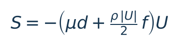
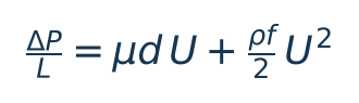
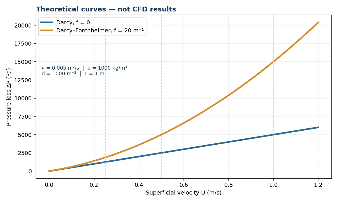
Here S is force per volume (N/m³), μ is dynamic viscosity (Pa s), ρ is density (kg/m³), d is the viscous coefficient (m⁻²), and f is the inertial coefficient (m⁻¹). For a nearly uniform steady one-dimensional flow through thickness L, the pressure loss attributable to the medium itself is approximately:
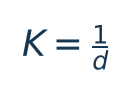
In the Darcy limit (f = 0) permeability is:
Caution: these are relations for the idealized constitutive model. They do not justify deriving K from two remote pressure readings in a domain with turns, entrance losses, bypass paths or free-flow regions.
Deep dive · How OpenFOAM 14 applies the law, line by line
From the description in DarcyForchheimer.H and from DarcyForchheimerTemplates.C:
D = diag(dx, dy, dz)            rotated into the coordinateSystem of the zone
F = 0.5 * diag(fx, fy, fz)      "leading 0.5 is from 1/2*rho"
Cd = mu*D + rho*|U|*F           per cell, |U| from the current velocity
Udiag   += V * tr(Cd)             implicit part (trace = 3c for isotropic Cd)
Usource -= V * (Cd - I*tr(Cd)) & U explicit correction- For an isotropic tensor Cd = c I the implicit part is 3c and the explicit correction −2c: at convergence exactly −c U remains. This “over-implicit” treatment makes the matrix more diagonally dominant and hence more stable with large resistances.
- In an incompressible case (kinematic pressure) the code uses ρ = 1 and μ = ν: the source is per unit mass, −(ν d + |U| f/2) U.
- Negative coefficients are not allowed as such: a negative value is read as a multiplier of the largest positive coefficient. The etc/caseDicts/fvModels/porosity/porousZone template uses this for a strongly anisotropic medium:
d (1e7 -1000 -1000);means 1·10⁷ in x and 1·10¹⁰ in y and z.
Deep dive · The campaign numbers (porous_estimates.py script)
| Case | K (m²) | ReK = U√K/ν | f U/(2 ν d) | ideal kinematic Δp (m²/s²) | ΔP (Pa, ρ = 1000) | τ = 1/(ν d + f U/2) | Co |
|---|---|---|---|---|---|---|---|
| obstacle_D0100 | 0.01 | 20 | 0 | 0.5 | 500 | 2 s | 0.40 |
| obstacle_D1000 | 0.001 | 6.3 | 0 | 5 | 5000 | 0.2 s | 0.40 |
| slab_D1000_F00_U025 | 0.001 | 1.6 | 0 | 1.25 | 1250 | 0.2 s | 0.10 |
| slab_D1000_F00_U100 | 0.001 | 6.3 | 0 | 5 | 5000 | 0.2 s | 0.40 |
| slab_D1000_F20_U025 | 0.001 | 1.6 | 0.5 | 1.875 | 1875 | 0.13 s | 0.10 |
| slab_D1000_F20_U100 | 0.001 | 6.3 | 2 | 15 | 15000 | 0.067 s | 0.40 |
The ratio f U/(2 ν d) measures the weight of the Forchheimer term against the Darcy term: it is 0.5, 1 and 2 at the three velocities with f = 20 m⁻¹, so the campaign crosses exactly the transition between the two regimes and is well designed to separate them by regression. ReK = U√K/ν is the permeability-based Reynolds number, used in the literature to mark the onset of inertial effects (order of magnitude 1–10). τ is the time with which the velocity in the zone adapts to a change: with 0.05 s steps the initial transient is over in a few steps. Values obtained by the script with the tutorial data; theoretical estimates, not CFD results.
python3 porous_estimates.py --manifest "$HOME/cases/guide14_campaign_01/manifest.csv" --ergun
python3 porous_estimates.py --profile exact_slab_F20_U100.csv --case slab_D1000_F20_U100
#!/usr/bin/env python3
# SPDX-License-Identifier: GPL-3.0-or-later
"""Order-of-magnitude checks and exact slab solution for the Guide 14 campaign.
Data of the OpenFOAM 14 porousBlockage tutorial: domain x -2..6 m, y -2..2 m,
64 x 32 x 1 cells (0.125 m), nu = 5e-3 m2/s, deltaT = 0.05 s, endTime = 100 s,
porous length L = 1 m. For every case of manifest.csv (or of the built-in
list) the script prints: permeability K = 1/d, Darcy number K/L^2,
Re_K = U sqrt(K)/nu, inertial/viscous ratio f U/(2 nu d), the ideal 1D
kinematic drop dp = (nu d U + f U^2/2) L and its value in Pa for the declared
rho, the momentum relaxation time 1/(nu d + f U/2) in the zone, the Courant
number and the flow-through time. --ergun inverts the Ergun relation used in
the guide (d = 150(1-e)^2/(e^3 dp^2), f = 3.5(1-e)/(e^3 dp)) for porosity e
and equivalent particle diameter dp. --profile writes a NEW csv with the
exact kinematic pressure p(x) of the slab case (uniform plug flow, symmetry
walls, outlet p = 0), comparable with a ParaView Plot Over Line export.
Theoretical values, not CFD results.
"""
import argparse
import csv
import math
from pathlib import Path
CASES = [('obstacle_D0100', 'obstacle', 100, 0, 1.0), ('obstacle_D0200', 'obstacle', 200, 0, 1.0),
('obstacle_D0500', 'obstacle', 500, 0, 1.0), ('obstacle_D1000', 'obstacle', 1000, 0, 1.0),
('slab_D1000_F00_U025', 'slab', 1000, 0, 0.25), ('slab_D1000_F00_U050', 'slab', 1000, 0, 0.5),
('slab_D1000_F00_U100', 'slab', 1000, 0, 1.0), ('slab_D1000_F20_U025', 'slab', 1000, 20, 0.25),
('slab_D1000_F20_U050', 'slab', 1000, 20, 0.5), ('slab_D1000_F20_U100', 'slab', 1000, 20, 1.0),
('slab_D0000_F00_U100', 'slab', 0, 0, 1.0)]
def ergun_inverse(d, f):
"""Porosity e and particle diameter dp from d [1/m2] and f [1/m] (guide's Ergun form)."""
e3 = 3.5 ** 2 * d / (150.0 * f * f) # d/f^2 = (150/12.25) e^3
e = e3 ** (1.0 / 3.0)
if not 0 < e < 1:
return None
dp = 3.5 * (1 - e) / (e3 * f)
return e, dp
def main():
p = argparse.ArgumentParser(description=__doc__, formatter_class=argparse.RawDescriptionHelpFormatter)
p.add_argument('--manifest', type=Path, help='manifest.csv of the campaign (default: built-in list)')
p.add_argument('--nu', type=float, default=5e-3)
p.add_argument('--rho', type=float, default=1000.0, help='declared reference density [kg/m3]')
p.add_argument('--L', type=float, default=1.0)
p.add_argument('--dx', type=float, default=0.125)
p.add_argument('--dt', type=float, default=0.05)
p.add_argument('--length', type=float, default=8.0, help='domain length [m]')
p.add_argument('--ergun', action='store_true')
p.add_argument('--profile', type=Path, help='NEW csv with exact slab p(x) for the case given by --case')
p.add_argument('--case', default='slab_D1000_F20_U100')
a = p.parse_args()
if a.manifest:
with a.manifest.open(newline='', encoding='utf-8') as h:
cases = [(r['case'], r['kind'], float(r['d_m_inv2']), float(r['f_m_inv']), float(r['U_m_s'])) for r in csv.DictReader(h)]
else:
cases = CASES
mu = a.rho * a.nu
print(f'mu = rho nu = {mu:g} Pa s (declared rho = {a.rho:g} kg/m3)')
print(f"{'case':22s} {'K [m2]':>9s} {'Da=K/L2':>8s} {'Re_K':>7s} {'fU/2nud':>8s} {'dp_kin':>8s} {'dp [Pa]':>9s} {'tau [s]':>8s} {'Co':>5s} {'T_flow':>7s}")
for name, kind, d, f, U in cases:
K = 1.0 / d if d > 0 else float('inf')
ratio = f * U / (2 * a.nu * d) if d > 0 else float('nan')
dpk = (a.nu * d * U + 0.5 * f * U * U) * a.L
res = a.nu * d + 0.5 * f * U
tau = 1.0 / res if res > 0 else float('inf')
reK = U * math.sqrt(K) / a.nu if d > 0 else float('inf')
print(f'{name:22s} {K:9.3g} {K / a.L ** 2:8.3g} {reK:7.3g} {ratio:8.3g} {dpk:8.4g} {a.rho * dpk:9.4g} {tau:8.3g} {U * a.dt / a.dx:5.2f} {a.length / U:7.3g}')
print('dp_kin = (nu d U + f U^2/2) L in m2/s2 (kinematic, as OpenFOAM p); dp [Pa] = rho dp_kin.')
print('For the obstacle cases dp is NOT the expected domain drop: the flow bypasses the block.')
if a.ergun:
print('\nErgun inversion (guide form, f term with the factor 1/2 of OpenFOAM):')
for d, f in sorted({(c[2], c[3]) for c in cases if c[2] > 0 and c[3] > 0}):
r = ergun_inverse(d, f)
print(f' d = {d:g} 1/m2, f = {f:g} 1/m -> ' + (f'porosity e = {r[0]:.3f}, dp = {r[1]:.4g} m' if r else 'no physical solution (e outside 0..1)'))
if a.profile:
if a.profile.exists():
p.error('profile output exists; refusing to overwrite')
sel = [c for c in cases if c[0] == a.case]
if not sel or sel[0][1] != 'slab':
p.error('--case must be a slab case of the list')
_, _, d, f, U = sel[0]
G = a.nu * d * U + 0.5 * f * U * U # kinematic gradient inside the zone
with a.profile.open('x', newline='', encoding='utf-8') as h:
w = csv.writer(h)
w.writerow(['x_m', 'p_exact_m2_s2', 'p_exact_Pa'])
for i in range(0, 601):
x = -1.5 + 3.0 * i / 600
pk = G * a.L if x <= -0.5 * a.L else (0.0 if x >= 0.5 * a.L else G * (0.5 * a.L - x))
w.writerow([f'{x:.5f}', f'{pk:.8g}', f'{a.rho * pk:.8g}'])
print(f'\nExact slab profile for {a.case}: p_up = {G * a.L:.6g} m2/s2, p_down = 0 -> written {a.profile}')
if __name__ == '__main__':
main()4. OpenFOAM pressure: check the physical dimensions
The source tutorial uses incompressibleFluid, and 0/p specifies dimensions [kinematicPressure]. The values displayed in ParaView therefore have units m²/s² rather than pascals. With a constant assumed reference density:
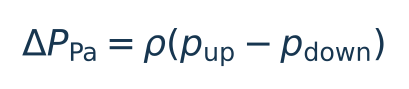
The tutorial sets nu = 5e-3 m²/s but needs no absolute density to solve its kinematic incompressible equations. This guide adopts ρ = 1000 kg/m³ as an explicit conversion assumption only, not as a CFD prediction. In general, μ = ρν.
OPTIONAL REVIEW — Pressure-loss sign. We define ΔP as upstream pressure minus downstream pressure. A negative result may imply reversed taps, the wrong reference or a physical situation requiring investigation. Always compare measurements from the same simulated time.
Deep dive · Kinematic pressure: units, reference and conversion
[kinematicPressure]is m²/s² (Pa divided by kg/m³). In ParaView and in thepostProcessingfiles the values are always kinematic.- The pressure level is fixed by the outlet,
p = 0: every value read is therefore a difference relative to the outlet. ThepRefCell 0; pRefValue 0;entries inPIMPLEplay no role, because a fixed-pressure boundary already exists. - For a real fluid choose ρ and set ν = μ/ρ in the case; the coefficients d and f do not change, because they are properties of the porous matrix. Example: water at 20 °C (μ ≈ 1.0·10⁻³ Pa s) with the same d = 1000 m⁻² would give a viscous resistance 5000 times smaller than in the teaching case.
foamDictionary 0/p -entry dimensions          # [kinematicPressure]
foamDictionary constant/physicalProperties -entry nu
Practical tip · Pascals directly in ParaView, without touching the data
- Calculator filter on the case: Attribute Type Cell Data (or Point Data), Result Array Name
p_Pa, expressionp*1000(declared ρ). The original kinematic field stays available for comparisons. - Plot Over Line from (−1.5, 0.0625, 0) to (1.5, 0.0625, 0) with Resolution 600: the same sampling as the
--profilefile ofporous_estimates.py, so the two CSV files can be compared column by column. - Write ρ in the field name or in the plot caption (for example “p_Pa, declared ρ = 1000 kg/m³”): whoever reads the plot a year later must know that the pascals do not come from the computation.
5. Official tutorial and case files
The verified reference is tutorials/incompressibleFluid/porousBlockage from the OpenFOAM/OpenFOAM-14 repository. Relevant files include system/blockMeshDict, system/createZonesDict, constant/fvModels, constant/coordinateSystems, constant/physicalProperties, 0/U, 0/p, and system/controlDict.
OpenFOAM Foundation 14 uses type porosityForce in constant/fvModels in this tutorial — not legacy fvOptions syntax from other releases. The following excerpt matches the Foundation-14 setup:
porosity
{
    type porosityForce;
    porosityForce
    {
        cellZone porousBlockage;
        type DarcyForchheimer;
        D 1000;
        d ($D $D $D);
        f (0 0 0);
        coordinateSystem porousBlockage;
    }
}
createZonesDict specifies a bounding box, and createZones assigns cells to the zone. The reference tutorial executes blockMesh, createZones, then foamRun. The preparation script supplied here copies the installed reference tutorial into new directories; the original is never modified.
Deep dive · createZones, coordinateSystems and model alternatives
createZonesreadssystem/createZonesDictand creates thecellZoneby selecting the cells whose centre lies in the box: check the zone cell count inlog.createZones(64 for the obstacle, 256 for the slab).constant/coordinateSystemsdefines the frame in which d and f are expressed (axesRotationwith e1 and e2). With isotropic coefficients the rotation is irrelevant; with a fibrous or channelled medium it matters a lot.- The version 14 porosityModel folder also contains
fixedCoeff(α, β coefficients with a reference density),powerLaw(ΔP ∝ |U|n) andsolidification;src/fvModels/interRegion/interRegionPorosityForceapplies the same force between regions.
The generic template etc/caseDicts/fvModels/porosity/porousZone shows the complete syntax with an in-dictionary coordinate system, a useful starting point for new cases.
6. Two geometries answer different questions
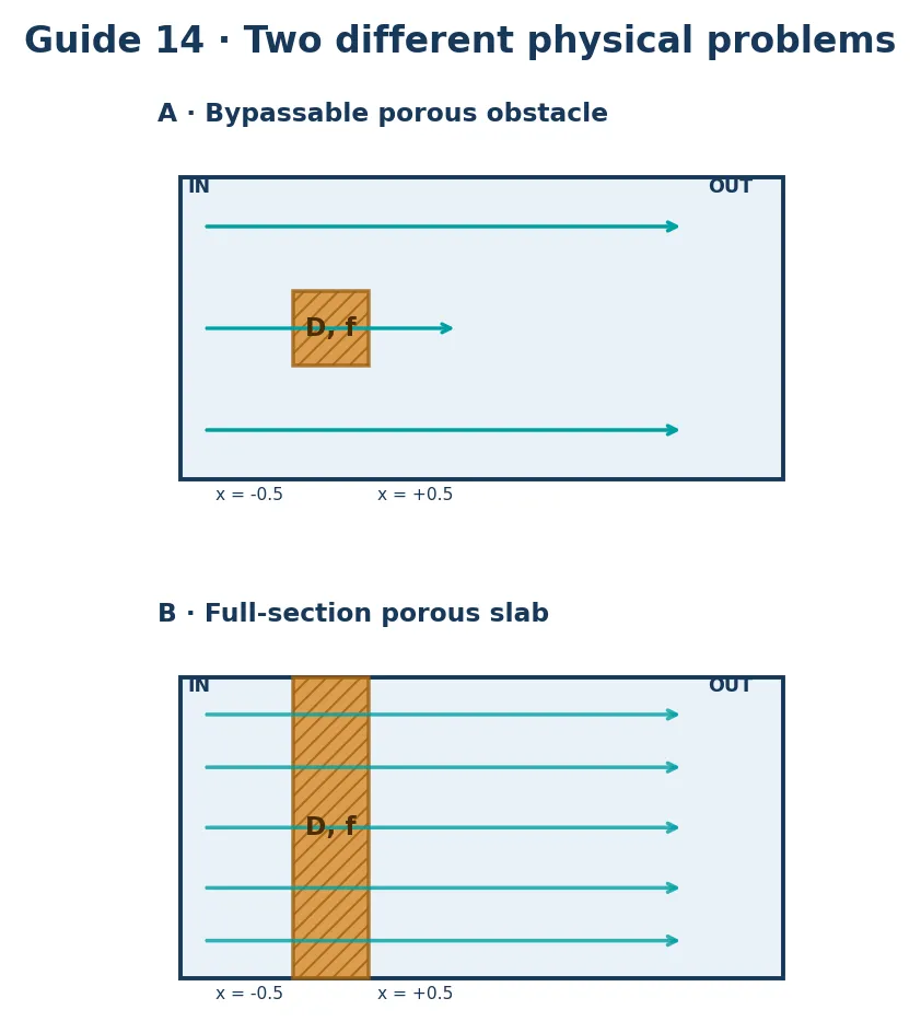
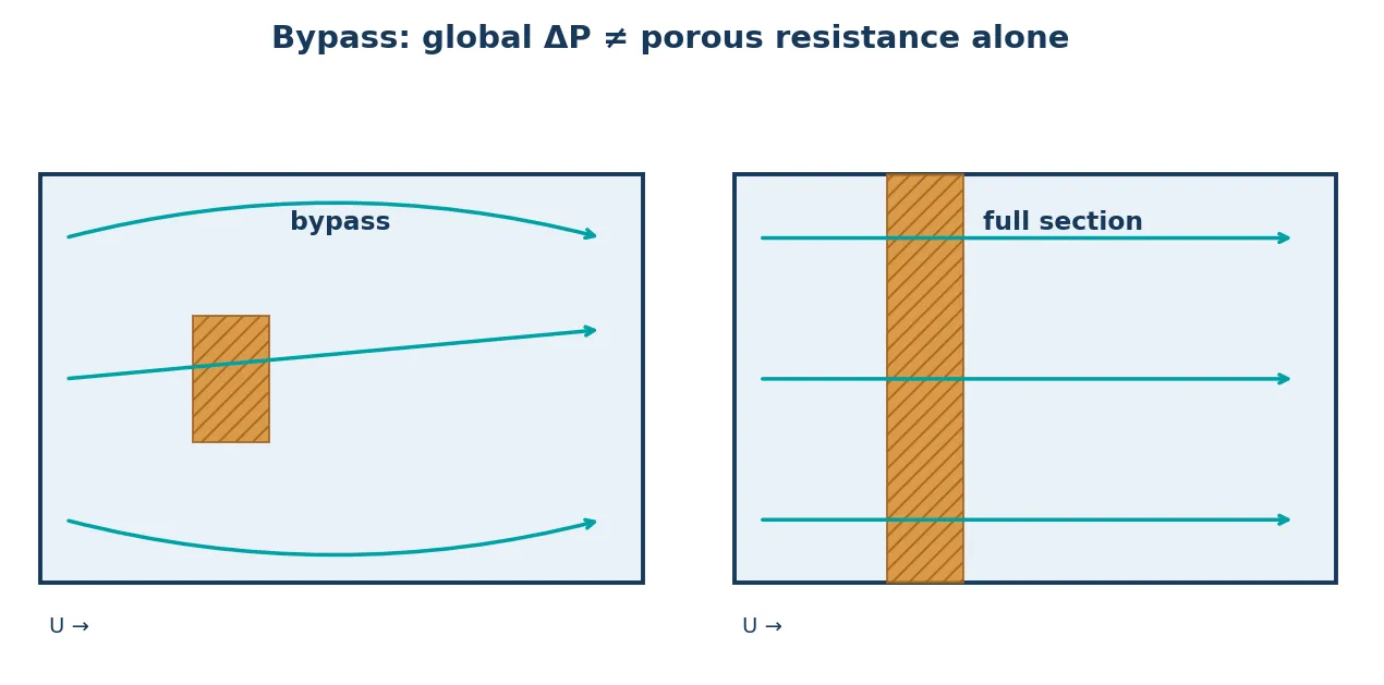
Configuration A — Bypassable obstacle. The porous region occupies −0.5 ≤ x ≤ 0.5 and −0.5 ≤ y ≤ 0.5 within a domain spanning −2 ≤ y ≤ 2. Flow can pass around the porous patch; the results illustrate redistribution, wakes and changes in d. The global pressure difference includes bypass and geometrical contributions, and does not directly determine 1D permeability.
Configuration B — Full-section porous slab. We extend the zone to −2.01 ≤ y ≤ 2.01, keeping porous length L = 1 m. The original upper and lower boundaries are symmetry planes. This arrangement greatly reduces bypass and permits a meaningful comparison of the average pressure gradient with Darcy–Forchheimer, provided numerical and inlet/outlet effects are also assessed.
Deep dive · How much flow actually crosses the obstacle
An order of magnitude follows from comparing the block resistance with the dynamic pressure pushing it. Crossing a block of length L requires Δp ≈ ν d L up (kinematic), while the pressure difference available between front and back of a bluff body is of the order of U²/2 … U². Hence up/U ≈ U/(ν d L):
| d (m⁻²) | ν d L (m/s) | estimated up/U |
|---|---|---|
| 100 | 0.5 | ≈ 1 (almost transparent block) |
| 200 | 1 | ≈ 0.5–1 |
| 500 | 2.5 | ≈ 0.2–0.4 |
| 1000 | 5 | ≈ 0.1–0.2 (almost impermeable) |
It is a rough estimate, but it explains why increasing d moves the flow to the side paths and why the global ΔP does not grow in proportion to d. The geometric blockage ratio is 1/4 (1 m out of a 4 m width): the two 1.5 m side paths accelerate the fluid up to about 4/3 U if the block is impermeable. Measuring the mean velocity inside the zone in ParaView (Threshold on the cellZone or Integrate Variables) and comparing it with this table is an excellent verification exercise.
Deep dive · The full-section slab has an exact solution
With a uniform inlet, symmetryPlane walls (no friction) and a zone spanning the whole section, the model solution is plug flow: U = Uin everywhere, p constant upstream and downstream, linear in the zone. With p = 0 at the outlet:
G = nu*d*U + f*U^2/2            (kinematic gradient in the zone, m/s2)
p(x) = G*L            for x <= -0.5
p(x) = G*(0.5 - x)     for -0.5 <= x <= 0.5
p(x) = 0              for x >= 0.5
In the finite-volume method the drop between the faces of each porous cell is G·Δx and free cells have no gradient: the drop between two free cells on either side of the zone is exactly G·L, independently of the mesh. Configuration B is therefore a code verification test with an exact solution: the expected deviation between measurement and formula is of the order of the solver tolerance. A deviation of a few per cent indicates a set-up error (zone, d, f, ν or U different from what you think), not a discretisation error. The porous_estimates.py --profile script writes this profile to a CSV comparable with Plot Over Line.
7. Prepare the campaign on Linux
Transfer the scripts folder from Windows using FileZilla. In PowerShell connect through SSH:
ssh USER@LINUX_SERVEREnable OpenFOAM 14 using the local installation’s normal environment script and check foamVersion, which blockMesh, which createZones, and which foamRun. Create the campaign in a new directory:
python3 prepare_campaign.py --output "$HOME/cases/guide14_campaign_01"If FOAM_TUTORIALS is not set, pass --source /path/to/tutorials/incompressibleFluid/porousBlockage. This operation needs no sudo, deletes nothing, and refuses an existing output folder. It creates one independent case per parameter set, a guide14_case.json file per case, and manifest.csv.
The campaign consists of 11 cases: four obstacles (d = 100, 200, 500, 1000 m⁻² at U = 1 m/s), six full-section slabs (d = 1000 m⁻², either f = 0 or 20 m⁻¹, at U = 0.25, 0.5, 1 m/s) and a zero-resistance control (d = f = 0).
Deep dive · Package script: prepare_campaign.py
It copies the installed tutorial into 11 new folders and, for each, replaces exactly once: the value of D and f in constant/fvModels; for the slabs, the zone name (porousSlab) in fvModels, createZonesDict and coordinateSystems and the box (-0.5 -2.01 -1) (0.5 2.01 1); the velocity in 0/U. It writes guide14_case.json, manifest.csv and README_FIRST.txt. Tested on the real OpenFOAM 14 tutorial: 11 cases created; the comparison with the original shows only the expected lines (for obstacle_D1000 the D line loses the “Fully shedding behavior” comment and f changes only in spacing). On error the partial folder is kept for diagnosis.
#!/usr/bin/env python3
# SPDX-License-Identifier: GPL-3.0-or-later
"""Prepare a non-destructive OpenFOAM-14 Darcy-Forchheimer campaign."""
import argparse
import csv
import json
import os
from pathlib import Path
import re
import shutil
import sys

CASES = [
    # Original porous obstacle: the lateral bypass invalidates a direct 1D Darcy fit.
    ('obstacle_D0100', 'obstacle', 100, 0, 1.0),
    ('obstacle_D0200', 'obstacle', 200, 0, 1.0),
    ('obstacle_D0500', 'obstacle', 500, 0, 1.0),
    ('obstacle_D1000', 'obstacle', 1000, 0, 1.0),
    # Cross-section-spanning porous slab: use for intrinsic resistance fitting.
    ('slab_D1000_F00_U025', 'slab', 1000, 0, 0.25),
    ('slab_D1000_F00_U050', 'slab', 1000, 0, 0.50),
    ('slab_D1000_F00_U100', 'slab', 1000, 0, 1.00),
    ('slab_D1000_F20_U025', 'slab', 1000, 20, 0.25),
    ('slab_D1000_F20_U050', 'slab', 1000, 20, 0.50),
    ('slab_D1000_F20_U100', 'slab', 1000, 20, 1.00),
    ('slab_D0000_F00_U100', 'slab', 0, 0, 1.00),
]

def replace_one(s: str, pattern: str, replacement: str, filename: str) -> str:
    new, n = re.subn(pattern, replacement, s, flags=re.MULTILINE)
    if n != 1:
        raise ValueError(f'{filename}: expected 1 editable entry, found {n}')
    return new

def modify_case(directory: Path, kind: str, d: int, f: int, speed: float) -> None:
    fv = directory / 'constant' / 'fvModels'
    src = fv.read_text(encoding='utf-8')
    src = replace_one(src, r'^(\s*)D\s+[0-9.eE+\-]+\s*;[^\n]*$', rf'\g<1>D {d};', str(fv))
    src = replace_one(src, r'^(\s*)f\s*\(\s*0\s+0\s+0\s*\)\s*;', rf'\g<1>f ({f} {f} {f});', str(fv))
    if kind == 'slab':
        src = replace_one(src, r'^\s*cellZone\s+porousBlockage\s*;', '        cellZone        porousSlab;', str(fv))
        src = replace_one(src, r'^\s*coordinateSystem\s+porousBlockage\s*;', '        coordinateSystem porousSlab;', str(fv))
    fv.write_text(src, encoding='utf-8')

    if kind == 'slab':
        zones = directory / 'system' / 'createZonesDict'
        z = zones.read_text(encoding='utf-8')
        z = replace_one(z, r'^porousBlockage\s*$', 'porousSlab', str(zones))
        z = replace_one(z, r'^\s*box\s*\([^\n]+;', '    box (-0.5 -2.01 -1) (0.5 2.01 1);', str(zones))
        zones.write_text(z, encoding='utf-8')
        systems = directory / 'constant' / 'coordinateSystems'
        cs = systems.read_text(encoding='utf-8')
        cs = replace_one(cs, r'^porousBlockage\s*$', 'porousSlab', str(systems))
        systems.write_text(cs, encoding='utf-8')

    ufile = directory / '0' / 'U'
    u = ufile.read_text(encoding='utf-8')
    u = replace_one(u, r'^internalField\s+uniform\s+\([^\n]*\);', f'internalField   uniform ({speed:g} 0 0);', str(ufile))
    ufile.write_text(u, encoding='utf-8')

    # The official Allrun is present only as provenance; execution uses run_campaign.sh.
    metadata = {'kind':kind,'d_m_inv2':d,'f_m_inv':f,'U_m_s':speed,
                'nu_m2_s':0.005,'porous_length_m':1.0,
                'pressure_units':'kinematic m2/s2','source':'OpenFOAM-14 porousBlockage'}
    (directory/'guide14_case.json').write_text(json.dumps(metadata, indent=2)+'\n', encoding='utf-8')

def main():
    ap = argparse.ArgumentParser(description=__doc__)
    ap.add_argument('--source', type=Path, default=None, help='Source OpenFOAM 14 porousBlockage tutorial directory')
    ap.add_argument('--output', type=Path, required=True, help='A NEW, non-existing campaign directory')
    args = ap.parse_args()
    source = args.source or Path(os.environ.get('FOAM_TUTORIALS',''))/'incompressibleFluid'/'porousBlockage'
    source = source.expanduser().resolve()
    target = args.output.expanduser().resolve()
    if not (source/'constant'/'fvModels').is_file():
        ap.error('OpenFOAM-14 porousBlockage tutorial not found; set --source or source OpenFOAM environment')
    if target.exists():
        ap.error(f'Output already exists (no overwrite): {target}')
    # Fail before writing if any required original file is missing.
    required = ['0/U','0/p','constant/coordinateSystems','constant/fvModels',
                'system/createZonesDict','system/blockMeshDict','system/controlDict']
    missing = [x for x in required if not (source/x).is_file()]
    if missing:
        ap.error('Missing required template files: '+', '.join(missing))
    target.mkdir(parents=True)
    try:
        manifest=[]
        for name, kind, d, f, vel in CASES:
            dest=target/name
            shutil.copytree(source,dest,symlinks=False)
            modify_case(dest,kind,d,f,vel)
            manifest.append({'case':name, 'kind':kind,'d_m_inv2':d, 'f_m_inv':f,'U_m_s':vel})
        with (target/'manifest.csv').open('w',newline='',encoding='utf-8') as h:
            w=csv.DictWriter(h,fieldnames=list(manifest[0]));w.writeheader();w.writerows(manifest)
        (target/'README_FIRST.txt').write_text('Source: '+str(source)+'\nNo CFD results exist yet. Run cases on OpenFOAM 14.\n',encoding='utf-8')
    except Exception:
        # Preserve partial output for diagnosis; never delete data automatically.
        print(f'ERROR: incomplete campaign preserved at {target}',file=sys.stderr)
        raise
    print(f'Created {len(manifest)} unique cases in: {target}')

if __name__=='__main__':
    main()
Practical tip · Quick checks after preparation
cd "$HOME/cases/guide14_campaign_01"
cat manifest.csv
for c in obstacle_D1000 slab_D1000_F20_U100; do
  echo "== $c"
  foamDictionary $c/constant/fvModels -entry porosity/porosityForce/cellZone
  foamDictionary $c/constant/fvModels -entry porosity/porosityForce/f
  grep -E "^ *box" $c/system/createZonesDict
  foamDictionary $c/0/U -entry internalField
done
The script writes manifest.csv with Windows line endings (CRLF, the default of Python’s csv module): run_campaign.sh reads the case name correctly, as it is the first field, but keep it in mind if you process the file with other Bash tools.
8. Run and monitor the simulations
Use tmux to protect a long run from an interrupted SSH session, as already discussed in Guide 1. Run a single case or the entire campaign:
bash run_campaign.sh "$HOME/cases/guide14_campaign_01" slab_D1000_F00_U025
# Entire campaign: bash run_campaign.sh "$HOME/cases/guide14_campaign_01"
Each run executes blockMesh, createZones, checkMesh, and foamRun sequentially. Logs are saved as log.blockMesh, log.createZones, log.checkMesh and log.foamRun. A guide14.SUCCESS marker merely indicates that the commands returned exit code zero; it does not mean the physics has been validated. Existing logs or failure markers prevent silent overwriting or automatic retries.
Review tail -n 50 log.foamRun and grep -Ei 'error|fatal|nan|floating|courant' log.foamRun. Download logs to Windows with FileZilla for further examination. Evaluate Courant number, mass conservation, transient behavior, and the stability of the physical quantities of interest.
Deep dive · WARNING: run_campaign.sh marks a failed case as successful
In the package script the commands run in a subshell written on the left of ||: in this position Bash disables set -e and the ERR trap inside the subshell. If blockMesh, createZones or foamRun fail, the script carries on with the following commands and the last one, touch guide14.SUCCESS, succeeds: the case is marked as successful and the script exits with code 0. Verified with stub commands simulating a failing foamRun: the guide14.SUCCESS marker is created and guide14.FAILED does not appear.
The corrected version run_campaign_fixed.sh (in the download, extra/ folder) chains the commands with && and decides the marker outside the subshell. Tested in the same three scenarios: failing foamRun → guide14.FAILED, exit code 1; failing blockMesh → stops immediately, only log.blockMesh, guide14.FAILED; all successful → guide14.SUCCESS, exit code 0. The same defect is present in the Guide 12 script, fixed the same way.
#!/usr/bin/env bash
# SPDX-License-Identifier: GPL-3.0-or-later
# Run the unmodified official OpenFOAM 14 applications in each prepared case.
# Corrected version of run_campaign.sh (Guide 14): failures are no longer marked as success.
set -euo pipefail
if [[ $# -lt 1 || $# -gt 2 ]]; then
  echo "Usage: bash run_campaign.sh CAMPAIGN_DIRECTORY [case_name]" >&2
  exit 2
fi
command -v blockMesh >/dev/null || { echo "Load OpenFOAM environment first." >&2; exit 2; }
command -v createZones >/dev/null || { echo "Missing createZones (OpenFOAM Foundation 14 required)." >&2; exit 2; }
command -v foamRun >/dev/null || { echo "Missing foamRun (OpenFOAM Foundation 14 required)." >&2; exit 2; }
root=$(realpath "$1")
[[ -f "$root/manifest.csv" ]] || { echo "Invalid campaign directory" >&2; exit 2; }
selected=${2:-}
found=0
while IFS=, read -r name kind d f speed; do
  [[ "$name" == 'case' ]] && continue
  [[ -n "$name" ]] || continue
  [[ -z "$selected" || "$name" == "$selected" ]] || continue
  found=1
  c="$root/$name"
  [[ -f "$c/guide14_case.json" ]] || { echo "Missing case metadata: $c" >&2; exit 1; }
  if [[ -f "$c/guide14.SUCCESS" ]]; then
    echo "SKIP completed: $name"
    continue
  fi
  if [[ -f "$c/guide14.FAILED" ]]; then
    echo "SKIP previously failed: $name (inspect logs; do not silently retry)"
    continue
  fi
  if [[ -e "$c/log.blockMesh" || -e "$c/log.createZones" || -e "$c/log.foamRun" ]]; then
    echo "SKIP existing logs: $name (manual inspection necessary)"
    continue
  fi
  echo "RUN $name"
  # Fix (Guide 14 article): a subshell on the left of || runs with errexit and the
  # ERR trap disabled, so the original version wrote guide14.SUCCESS even when a
  # command failed. Each step is now chained with && and checked explicitly.
  if ( cd "$c" &&
       blockMesh > log.blockMesh 2>&1 &&
       createZones > log.createZones 2>&1 &&
       checkMesh > log.checkMesh 2>&1 &&
       foamRun > log.foamRun 2>&1 ); then
    touch "$c/guide14.SUCCESS"
  else
    touch "$c/guide14.FAILED"
    echo "FAILED $name; inspect case logs" >&2
    exit 1
  fi
done < "$root/manifest.csv"
[[ "$found" == 1 ]] || { echo "No matching case name" >&2; exit 2; }
Deep dive · Package script: run_campaign.sh (original)
Reproduced in full as in the package. It checks the environment (blockMesh, createZones, foamRun), skips cases already completed, failed or with existing logs and deletes nothing; for the marker defect see the previous box.
#!/usr/bin/env bash
# SPDX-License-Identifier: GPL-3.0-or-later
# Run the unmodified official OpenFOAM 14 applications in each prepared case.
set -euo pipefail
if [[ $# -lt 1 || $# -gt 2 ]]; then
  echo "Usage: bash run_campaign.sh CAMPAIGN_DIRECTORY [case_name]" >&2
  exit 2
fi
command -v blockMesh >/dev/null || { echo "Load OpenFOAM environment first." >&2; exit 2; }
command -v createZones >/dev/null || { echo "Missing createZones (OpenFOAM Foundation 14 required)." >&2; exit 2; }
command -v foamRun >/dev/null || { echo "Missing foamRun (OpenFOAM Foundation 14 required)." >&2; exit 2; }
root=$(realpath "$1")
[[ -f "$root/manifest.csv" ]] || { echo "Invalid campaign directory" >&2; exit 2; }
selected=${2:-}
found=0
while IFS=, read -r name kind d f speed; do
  [[ "$name" == 'case' ]] && continue
  [[ -n "$name" ]] || continue
  [[ -z "$selected" || "$name" == "$selected" ]] || continue
  found=1
  c="$root/$name"
  [[ -f "$c/guide14_case.json" ]] || { echo "Missing case metadata: $c" >&2; exit 1; }
  if [[ -f "$c/guide14.SUCCESS" ]]; then
    echo "SKIP completed: $name"
    continue
  fi
  if [[ -f "$c/guide14.FAILED" ]]; then
    echo "SKIP previously failed: $name (inspect logs; do not silently retry)"
    continue
  fi
  if [[ -e "$c/log.blockMesh" || -e "$c/log.createZones" || -e "$c/log.foamRun" ]]; then
    echo "SKIP existing logs: $name (manual inspection necessary)"
    continue
  fi
  echo "RUN $name"
  (
    cd "$c"
    trap 'touch guide14.FAILED' ERR
    blockMesh > log.blockMesh 2>&1
    createZones > log.createZones 2>&1
    checkMesh > log.checkMesh 2>&1
    foamRun > log.foamRun 2>&1
    touch guide14.SUCCESS
  ) || { echo "FAILED $name; inspect case logs" >&2; exit 1; }
done < "$root/manifest.csv"
[[ "$found" == 1 ]] || { echo "No matching case name" >&2; exit 2; }
Deep dive · Measuring during the run: a system/functions file for porous media
The tutorial has no system/functions. The following file (with the FoamFile header, essential in OpenFOAM 14) records at every step pressure and velocity at five probes (cell centres, because y = 0 lies on a face), the mean inlet pressure, the inlet and outlet flow rates for the mass balance and, from t = 20 s, the time averages of U and p. Copy it into system/functions of each case before the run.
/*--------------------------------*- C++ -*----------------------------------*\
  Guide 14 - monitoring functions for a NEW copy of a porousBlockage case.
  Save as <case>/system/functions BEFORE run_campaign.sh.
  The FoamFile header is required: without it OpenFOAM 14 ignores the file.
\*---------------------------------------------------------------------------*/
FoamFile
{
    format      ascii;
    class       dictionary;
    location    "system";
    object      functions;
}

// Pressure taps (kinematic p) and velocity on the channel axis, every time step.
// All points are cell centres of the 0.125 m mesh (y = 0 and y = 0.75 would lie on
// faces): x = -1.5625 far upstream, -0.5625 and +0.5625 first free cells next to
// the porous zone, +1.5625 far downstream; (2.5625 0.8125) lies in the wake and is
// used for the shedding frequency (probe index 4).
#includeFunc probes
(
    name=pressureTaps,
    points=((-1.5625 0.0625 0) (-0.5625 0.0625 0) (0.5625 0.0625 0) (1.5625 0.0625 0) (2.5625 0.8125 0)),
    fields=(p U)
)

// Area-averaged pressure on the inlet (the outlet is fixed at p = 0)
#includeFunc patchAverage(name=pInlet, patch=inlet, fields=(p))

// Volumetric flow rates [m3/s] for the mass balance (inlet negative, outlet positive)
#includeFunc patchFlowRate(name=Qinlet, patch=inlet)
#includeFunc patchFlowRate(name=Qoutlet, patch=outlet)

// Time averages after the initial transient (shedding cases)
#includeFunc fieldAverage(fields=(U p), startTime=20)

// ************************************************************************* //
for c in $(tail -n +2 "$HOME/cases/guide14_campaign_01/manifest.csv" | cut -d, -f1); do
cp -n functions_guide14 "$HOME/cases/guide14_campaign_01/$c/system/functions"
donePractical tip · Duration, time step and steady cases
- 2048 cells and 2000 steps (100 s with Δt = 0.05 s): from a few seconds to a few minutes per case on one core; the 11 cases in sequence stay light.
- The step is fixed (no
adjustTimeStep): Co = U Δt/Δx = 0.4 with U = 1 m/s, up to about 0.55 in the accelerated side paths. - The slabs reach steady state in a few steps (τ ≤ 0.2 s): a few simulated seconds are enough for them; still keep the same
endTimefor a homogeneous campaign, or document the reduction in a copy. - In the log, the
time step continuity errorsline must stay small and theGAMGiterations on p must not grow over time.
9. Exercise A — A porous obstacle with bypass
Open each case in ParaView using pvserver; visualize U, p, slices, and streamlines at comparable physical times for each d. Record the peak bypass speed, wake extent and any unsteadiness. Higher porous resistance may route more fluid around the patch; thus the difference between remote taps cannot be expected to scale linearly with d.
Deliverable: four views on a common color scale, an observation table, and a short discussion of recirculation. For oscillatory or transient flow, compare time averages after the initial transient rather than unrelated individual frames.
Deep dive · Time averages, shedding frequency and Strouhal number (probe_series.py script)
For cases with a periodic wake, quantities must be averaged over an integer number of periods, after the transient. With the functions file of the section 8 box, fieldAverage writes UMean and pMean (useful in ParaView), while the following script reads the probes and returns mean, standard deviation, minimum and maximum of the pressure difference between two taps and the dominant frequency of a velocity component (zero crossings of the fluctuation). The Strouhal number St = f D/U of a bluff body at Re ≈ 200 is of the order of 0.15–0.2; a porous block, partly crossed by the flow, tends to different values and a shorter wake.
Tested on synthetic series: imposed frequency 0.21 Hz recovered exactly (16 periods), mean pressure difference 4.9997 m²/s² with an imposed oscillation. With --fill it writes the measurement CSV for analyze_pressure.py directly from the time-averaged tap values, as an alternative to the manual filling described in section 11.
cd "$HOME/cases/guide14_campaign_01"
python3 probe_series.py obstacle_D*/postProcessing/pressureTaps/0/p --tstart 20 --U --probe-u 4 --component 1 --D 1 --uref 1
#!/usr/bin/env python3
# SPDX-License-Identifier: GPL-3.0-or-later
"""Pressure-tap statistics from OpenFOAM 14 probes files (Guide 14).
Reads postProcessing/<probes name>/<time>/p of one or more cases (scalar
probes, one column per point, comment lines starting with '#') and, for
t >= --tstart, prints mean, standard deviation, minimum and maximum of the
kinematic difference p[up] - p[down] and its value in Pa (declared --rho).
With --U the matching U file is read as well and the dominant frequency of
the chosen component at --probe-u is estimated from upward zero crossings of
the fluctuation (mean removed); the Strouhal number St = freq * D / U_ref
is printed with --D and --uref. With --fill a NEW csv is written with the
columns case,p_up_m2_s2,p_down_m2_s2 expected by analyze_pressure.py,
using the time-averaged tap values.
"""
import argparse
import csv
import math
from pathlib import Path
import statistics as st
import sys
def read_probes(path):
t, rows = [], []
with open(path, encoding='utf-8') as f:
for line in f:
s = line.strip()
if not s or s.startswith('#'):
continue
parts = s.replace('(', ' ').replace(')', ' ').split()
vals = [float(x) for x in parts]
t.append(vals[0])
rows.append(vals[1:])
if not t:
raise ValueError(f'{path}: no data rows')
return t, rows
def zero_cross_freq(t, y):
m = st.fmean(y)
ups = [t[i - 1] + (t[i] - t[i - 1]) * (m - y[i - 1]) / (y[i] - y[i - 1])
for i in range(1, len(y)) if y[i - 1] < m <= y[i]]
if len(ups) < 3:
return None, len(ups)
periods = [b - a for a, b in zip(ups, ups[1:])]
return 1.0 / st.fmean(periods), len(periods)
def main():
p = argparse.ArgumentParser(description=__doc__, formatter_class=argparse.RawDescriptionHelpFormatter)
p.add_argument('pfiles', type=Path, nargs='+', help='probes p files, e.g. CASE/postProcessing/pressureTaps/0/p')
p.add_argument('--up', type=int, default=1, help='index of the upstream tap (0-based)')
p.add_argument('--down', type=int, default=2, help='index of the downstream tap (0-based)')
p.add_argument('--tstart', type=float, default=0.0)
p.add_argument('--rho', type=float, default=1000.0)
p.add_argument('--U', action='store_true', help='also analyse the U probes file next to each p file')
p.add_argument('--probe-u', type=int, default=4, help="probe index for the frequency analysis")
p.add_argument('--component', type=int, default=1, help='0 = Ux, 1 = Uy, 2 = Uz')
p.add_argument('--D', type=float, default=1.0, help='reference length for Strouhal [m]')
p.add_argument('--uref', type=float, default=1.0, help='reference velocity for Strouhal [m/s]')
p.add_argument('--fill', type=Path, help='NEW measurements csv for analyze_pressure.py')
a = p.parse_args()
if a.fill and a.fill.exists():
p.error('--fill output exists; refusing to overwrite')
out = []
for f in a.pfiles:
case = f.parts[-5] if len(f.parts) >= 5 else f.stem
t, rows = read_probes(f)
sel = [(ti, r) for ti, r in zip(t, rows) if ti >= a.tstart]
if len(sel) < 2:
p.error(f'{f}: fewer than 2 records after t = {a.tstart}')
up = [r[a.up] for _, r in sel]
dn = [r[a.down] for _, r in sel]
dp = [u - d for u, d in zip(up, dn)]
m, s = st.fmean(dp), (st.pstdev(dp) if len(dp) > 1 else 0.0)
print(f'{case}: {len(sel)} records, t = {sel[0][0]:g}..{sel[-1][0]:g} s')
print(f' p_up mean {st.fmean(up):.6g}, p_down mean {st.fmean(dn):.6g} m2/s2')
print(f' dp = {m:.6g} +- {s:.3g} m2/s2 (min {min(dp):.6g}, max {max(dp):.6g}) -> {a.rho * m:.6g} +- {a.rho * s:.3g} Pa')
out.append((case, st.fmean(up), st.fmean(dn)))
if a.U:
tu, ru = read_probes(f.with_name('U'))
k = 3 * a.probe_u + a.component
selu = [(ti, r[k]) for ti, r in zip(tu, ru) if ti >= a.tstart]
fr, n = zero_cross_freq([x for x, _ in selu], [y for _, y in selu])
if fr:
print(f' U component {a.component} at probe {a.probe_u}: frequency {fr:.4g} Hz over {n} periods, St = {fr * a.D / a.uref:.4g}')
else:
print(f' U component {a.component} at probe {a.probe_u}: no periodic signal detected (steady or too short)')
if a.fill:
with a.fill.open('x', newline='', encoding='utf-8') as h:
w = csv.writer(h)
w.writerow(['case', 'p_up_m2_s2', 'p_down_m2_s2'])
for c, u, d in out:
w.writerow([c, f'{u:.8g}', f'{d:.8g}'])
print('Written', a.fill)
if __name__ == '__main__':
try:
main()
except (OSError, ValueError) as exc:
sys.exit(f'ERROR: {exc}')Practical tip · Comparable views in ParaView
- Same scale for all cases:
Ufrom 0 to 1.5 m/s,pwith a fixed range chosen on the highest-resistance case. - To see the zone:
Extract Blockor, in the reader, selecting theporousBlockagecellZone(“Read zones” option). Stream Tracerwith a line seed on the inlet (from (−2, −1.9) to (−2, 1.9)): it shows the fraction of streamlines crossing the block.- For periodic cases use
UMeanandpMeanat the last time instead of the instantaneous fields.
10. Exercise B — A full slab in the Darcy limit
Open slab_D1000_F00_U*. In ParaView use Plot Over Line along the centerline from (-1.5,0,0) to (1.5,0,0), retaining identical sampling points for every speed. Export p(x) to CSV. The gradient should be approximately constant within the porous zone and weak outside it, apart from discrete interface effects.
For a simple point-tap estimate, sample immediately outside the slab, for example at x = −0.625 m and +0.625 m (with y = 0). These are approximate pressure-loss measurements, not a metrologically exact extraction of intrinsic permeability. A stronger procedure estimates the pressure gradient from the interior of the zone and checks the sensitivity to mesh and tap position.
Theoretical prediction only: with ν = 0.005 m²/s, ρ = 1000 kg/m³, d = 1000 m⁻², L = 1 m and f = 0, the 1D model predicts approximately 1250, 2500 and 5000 Pa at 0.25, 0.5 and 1 m/s. These are not CFD results.
Deep dive · What exactly to expect in this experience
For the exact solution of the section 6 box, with p = 0 at the outlet, the expected tap values are:
| Case | p_up (m²/s²) | p_down (m²/s²) | ΔP (Pa, ρ = 1000) |
|---|---|---|---|
| slab_D1000_F00_U025 | 1.25 | 0 | 1250 |
| slab_D1000_F00_U050 | 2.5 | 0 | 2500 |
| slab_D1000_F00_U100 | 5 | 0 | 5000 |
| slab_D1000_F20_U025 | 1.875 | 0 | 1875 |
| slab_D1000_F20_U050 | 5 | 0 | 5000 |
| slab_D1000_F20_U100 | 15 | 0 | 15000 |
| slab_D0000_F00_U100 | 0 | 0 | 0 |
In this specific case, therefore, p_down ≈ 0 and p_up equals the drop across the slab. The x = ±0.625 m points suggested by the guide lie on mesh faces (cell centres are at ±0.5625 and ±0.6875): ParaView interpolates the values to the points and, since pressure is constant in the free regions, the result does not change. The package’s measurement_example_SYNTHETIC.csv file, on the other hand, has non-zero p_down values: it is a mathematical example to test the script, not a prediction of the simulation.
Practical tip · Slope inside the zone instead of two points
With Plot Over Line from (−1.5, 0.0625, 0) to (1.5, 0.0625, 0) and resolution 1200 you get p(x); a least-squares line on the points with −0.4 < x < 0.4 only gives the slope G = −dp/dx, independent of the reference level. Comparing G·L with the difference between the two outer points measures edge effects. Alternatively foamPostProcess -func "graphCell(name=axis, start=(-1.5 0.0625 0), end=(1.5 0.0625 0), axis=x, fields=(p U))" writes one point per cell, with no interpolation.
11. Exercise C — Forchheimer and curve fitting
Repeat the extraction for slab_D1000_F20_U*, with f = 20 m⁻¹. The quadratic pressure contribution increases with velocity. The ideal 1D model predicts 1875, 5000 and 15000 Pa for the same three flow speeds. Again, these numbers are theoretical rather than measured.
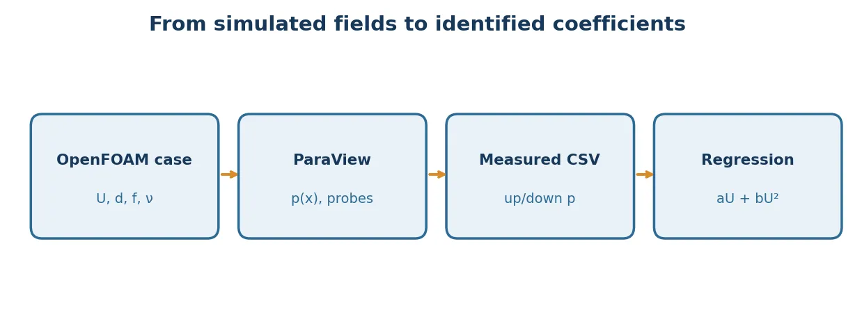
Once you have extracted actual CFD values, sample the same two locations and manually fill in measurements_template.csv using the columns case,p_up_m2_s2,p_down_m2_s2. Save the completed file under a new name such as measured_pressures.csv. The tool deliberately does not guess which ParaView columns or taps are physically appropriate. Then run:
python3 analyze_pressure.py \
  --manifest "$HOME/cases/guide14_campaign_01/manifest.csv" \
  --measurements measured_pressures.csv \
  --output pressure_results.csv --rho 1000
The script refuses existing output paths and duplicate case records. Provided at least three distinct speeds are present, it fits ΔP/L = a U + b U² using least squares. It then estimates d = a/μ and f = 2b/ρ, with μ = ρν. Fitting is a diagnostic step: it is not by itself proof that the 1D assumptions are valid.
Deep dive · Package script: analyze_pressure.py
It reads the manifest and the measurement CSV, rejects duplicates, unknown cases, non-finite values and existing output files; converts to Pa with the declared ρ, compares with the 1D slab prediction and, for the slabs with d = 1000 m⁻², fits for each value of f the least-squares relation ΔP/L = aU + bU² without intercept by solving the 2 × 2 normal equations. Tested with the package’s synthetic file: it recovers exactly d = 1000 m⁻² and f = 0 for the first group, d = 1000 m⁻² and f = 20 m⁻¹ for the second, with zero differences from the ideal prediction.
Warning: the script uses fixed values ν = 0.005 m²/s and L = 1 m (lines d_est_m_inv2 = a/(rho*0.005) and L=1.0; nu=0.005). If the case viscosity or the slab thickness is changed, these two numbers must be changed too, otherwise the estimated d and the ideal prediction are wrong.
#!/usr/bin/env python3
# SPDX-License-Identifier: GPL-3.0-or-later
"""Analyze measured ParaView kinetic-pressure taps and Darcy-Forchheimer fit.

Input CSV columns: case,p_up_m2_s2,p_down_m2_s2
This script does NOT read OpenFOAM fields automatically and does NOT fabricate CFD data.
"""
import argparse
import csv
import math
from pathlib import Path


def calc_fit(samples, rho, length):
    # Least squares: deltaP/L = a U + b U^2. No intercept by physical model.
    if len(samples)<3 or len({u for u,_ in samples})<3:
        return None
    s2=sum(u*u for u,y in samples)
    s3=sum(u**3 for u,y in samples)
    s4=sum(u**4 for u,y in samples)
    r1=sum(u*y/length for u,y in samples)
    r2=sum(u*u*y/length for u,y in samples)
    det=s2*s4-s3*s3
    if abs(det)<1e-20:
        return None
    a=(r1*s4-r2*s3)/det
    b=(r2*s2-r1*s3)/det
    return {'a_Pa_s_m2':a,'b_Pa_s2_m3':b,'d_est_m_inv2':a/(rho*0.005),
            'f_est_m_inv':2*b/rho}

def main():
    ap=argparse.ArgumentParser(description=__doc__)
    ap.add_argument('--manifest',type=Path,required=True)
    ap.add_argument('--measurements',type=Path,required=True)
    ap.add_argument('--output',type=Path,required=True)
    ap.add_argument('--rho',type=float,default=1000., help='Assumed reference density [kg/m3]')
    args=ap.parse_args()
    if args.rho<=0:ap.error('rho must be positive')
    if args.output.exists():ap.error('output already exists; refusal to overwrite')
    with args.manifest.open(newline='',encoding='utf-8') as h:
        manifest={r['case']:r for r in csv.DictReader(h)}
    with args.measurements.open(newline='',encoding='utf-8') as h:
        measurements=list(csv.DictReader(h))
    if not measurements:ap.error('No real measurement rows. Fill the CSV after ParaView extraction.')
    rows=[]; seen=set(); fit_groups={}
    for row in measurements:
        name=row['case']
        if name in seen:ap.error('Duplicate case measurement: '+name)
        seen.add(name)
        if name not in manifest:ap.error('Unknown case: '+name)
        m=manifest[name]
        try:
            up=float(row['p_up_m2_s2']);down=float(row['p_down_m2_s2'])
        except (KeyError,ValueError):ap.error('Missing or invalid kinetic pressures for '+name)
        if not all(map(math.isfinite,[up,down])):ap.error('Non-finite pressures: '+name)
        u=float(m['U_m_s']); d=float(m['d_m_inv2']); f=float(m['f_m_inv']); L=1.0; nu=0.005
        dp=args.rho*(up-down)
        theoretical=args.rho*L*(nu*d*u+0.5*f*u*u)
        rec={'case':name,'kind':m['kind'],'U_m_s':u,'d_m_inv2':d,'f_m_inv':f,
             'deltaP_measured_Pa':dp,'deltaP_ideal_slab_Pa':theoretical,
             'difference_Pa':dp-theoretical}
        rows.append(rec)
        if m['kind']=='slab' and d==1000:
            fit_groups.setdefault(f,[]).append((u,dp))
    args.output.parent.mkdir(parents=True,exist_ok=True)
    with args.output.open('w',newline='',encoding='utf-8') as h:
        w=csv.DictWriter(h,fieldnames=list(rows[0]));w.writeheader();w.writerows(rows)
    print('Output:',args.output,'--',len(rows),'real measurements')
    for f, vals in sorted(fit_groups.items()):
        fit=calc_fit(vals,args.rho,1.0)
        if fit:
            print(f'Fit for f specified {f:g} 1/m:',', '.join(f'{k}={v:.6g}' for k,v in fit.items()))
        else: print(f'Not enough distinct velocities for f={f:g} fit')
    print('NOTE: Ideal slab predictions omit entrances, axial development and numerical errors.')
    print('NOTE: Obstacle measurements are not eligible for 1D intrinsic K estimation.')

if __name__=='__main__':main()
Deep dive · How reliable is a regression on three velocities
With three points and two parameters only one degree of freedom remains to estimate the error: the regression determines a and b but not their uncertainty robustly. Advice: use 5–7 velocities distributed so that f U/(2 ν d) goes from about 0.1 to 3; report the residual of each point; check that the f = 0 group returns b ≈ 0 (a free internal check); compare with the dimensionless representation ΔP/(L μ U) = d + (ρ f/2μ) U, which is a straight line in U and reveals any unexpected term.
Deep dive · Package example files
Full text of the two files in the examples/ folder: the empty template to fill in and the synthetic example (mathematical test values, not CFD results).
examples/measurements_template.csv
case,p_up_m2_s2,p_down_m2_s2examples/measurement_example_SYNTHETIC.csv
case,p_up_m2_s2,p_down_m2_s2
slab_D1000_F00_U025,2.02,0.77
slab_D1000_F00_U050,3.15,0.65
slab_D1000_F00_U100,6.14,1.14
slab_D1000_F20_U025,2.785,0.91
slab_D1000_F20_U050,6.30,1.30
slab_D1000_F20_U100,16.20,1.20
12. Permeability, porosity and the Ergun relation
Within the Darcy model, intrinsic permeability is K = 1/d. To relate the resistance of an idealized granular bed to particle equivalent diameter d_p and void fraction ε, the Ergun correlation gives (under its geometric and flow-regime assumptions):
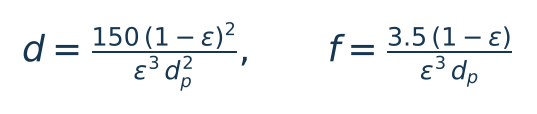
Do not apply this relation without justification to expanded metal, anisotropic networks, microstructured materials, or non-Newtonian fluids. For anisotropic media, resistance is directional and the coordinateSystems orientation matters. The provided cases are isotropic: d = (D D D) and f = (F F F).
OPTIONAL REVIEW — Dimensions. [d] = m⁻², [f] = m⁻¹, [K] = m². Void fraction ε and ECSA surface-area ratios are dimensionless, but they neither equal one another nor uniquely determine permeability.
Deep dive · Ergun in OpenFOAM form and inversion for the campaign parameters
The Ergun correlation (Chem. Eng. Prog. 48, 1952) reads ΔP/L = 150 μ(1−ε)²U/(ε³dp²) + 1.75 ρ(1−ε)U²/(ε³dp). Comparing it with μ d U + ρ f U²/2 gives the coefficient 150 for d and 2 × 1.75 = 3.5 for f: the guide’s factor 3.5 accounts for the ½ by which OpenFOAM multiplies f. Inverting the two relations:
d / f^2 = (150 / 3.5^2) * eps^3    ->  eps^3 = 12.25 d / (150 f^2)
d_p    = 3.5 (1 - eps) / (eps^3 f)
For d = 1000 m⁻² and f = 20 m⁻¹ one gets ε ≈ 0.589 and dp ≈ 0.35 m (porous_estimates.py --ergun script): the teaching coefficients correspond to a bed of 35 cm spheres, not to a filter. The inverse calculation is a good plausibility check when d and f are received from third parties. Known variants: Macdonald et al. (Ind. Eng. Chem. Fundam. 18, 1979) propose 180 and 1.8–4; the Kozeny–Carman relation coincides with the viscous term alone with constant 180.
Practical tip · Anisotropic coefficients in practice
// honeycomb or straightener aligned with x: low resistance along the channels,
// almost blocked across them (negative = multiplier of the largest coefficient)
d   (1000 -1000 -1000);     // -> 1000, 1e6, 1e6 1/m2
f   (0 0 0);
coordinateSystem porousBlockage;   // e1 = flow direction
Rotating e1 in constant/coordinateSystems aligns the “easy” direction with the material channels. With very high resistance ratios convergence often needs a smaller step.
Practical tip · Particle Reynolds number: is the campaign within Ergun’s range?
The modified bed Reynolds number is Rep = ρ U dp / (μ (1 − ε)) = U dp / (ν (1 − ε)). With ε = 0.589 and dp = 0.3524 m obtained above and ν = 0.005 m²/s:
| U [m/s] | Rep | regime |
|---|---|---|
| 0.25 | ≈ 43 | transitional: both terms matter |
| 0.50 | ≈ 86 | transitional |
| 1.00 | ≈ 171 | inertia dominant |
Ergun derived the correlation from data with Rep up to a few thousand; below Rep ≈ 10 the viscous term dominates (Kozeny–Carman), above a few hundred the quadratic term does. The ratio between the two terms, 1.75 Rep/150, equals 1 at Rep ≈ 86: exactly the intermediate velocity of the campaign, which is why the three chosen velocities separate a and b well. If a real medium works at Rep < 1, the f term becomes invisible in the regression: there is no point estimating it.
13. Numerical verification and uncertainty
Never accept a fit solely because it has a high R². Check checkMesh, boundary patches and a ParaView rendering of the cellZone. Confirm consistent inlet and outlet mass flow; compare mesh resolutions (for example, doubling two mesh directions); vary sample location; wait until a steady condition is reached or average an established transient; verify that pressure is kinematic; and repeat the study across multiple velocities. Three-dimensional heterogeneous flows are better represented by cross-section averages than by single-point taps.
The full slab is suitable for estimating K only when flow actually crosses it without bypass and external losses are measured or accounted for. The d = f = 0 control helps estimate background pressure loss but does not replace grid-convergence assessment.
Deep dive · Concrete numerical verification plan
- Code verification: slab with f = 0 and f = 20 compared with the exact solution (section 6); expected deviation of the order of the tolerance.
- Mass balance:
Qinlet+Qoutlet≈ 0 from thepostProcessingfiles (flow rates in m³/s for the 0.2 m thickness; Q = 0.8 m³/s with U = 1). - Mesh: in a copy,
(64 32 1)→(128 64 1)inblockMeshDict(zone limits stay on faces) and Δt halved to keep the Courant number; for the obstacle compare the mean ΔP and the shedding frequency. - Time: Δt = 0.025 s in a copy; for averages, different windows (20–100 s and 50–100 s) must give the same value within the uncertainty.
- Reference: the
slab_D0000_F00_U100case must give p ≈ 0 everywhere; a non-zero value indicates a background loss of the domain or a set-up error.
For discretisation uncertainty and the Grid Convergence Index see Guide 4.
14. Filters, catalytic beds and expanded-metal structures
The same approach gives a first equivalent model of a filter, a catalytic support or a monolith if its thickness and coordinate orientation are defined. For expanded metal, comparing a pore-resolved geometry with an equivalent porous resistance requires calibration against flow rate and pressure drop under several operating conditions. An area ratio such as SEF or ECSA alone cannot determine d or f. Reactive transport and species transfer require additional models that are outside this guide.
Deep dive · From the laboratory test to the model coefficients
- Measure ΔP on a sample of known thickness L at 5–7 flow rates, with pressure taps away from the sample faces and an empty test (without sample) to subtract.
- Compute the superficial velocity U = Q/A with the total cross-section area, the same definition OpenFOAM uses.
- Fit ΔP/L = aU + bU² with the same fluid and temperature; d = a/μ, f = 2b/ρ (exactly as in
analyze_pressure.py). - Insert d and f in the model and check with a full-section case (like this guide’s slab) that the simulation reproduces the measurements: this is calibration; validation then requires a geometry different from the calibration one.
For a complete treatment of macroscopic models: Nield and Bejan, Convection in Porous Media, 5th ed., Springer 2017, chapter 1.
Deep dive · What the model does not know: porosity, residence times and transport
- The
porosityForcefvModel only adds a force to the momentum equation: porosity ε appears in no other equation. The computed velocity is the superficial one; the real interstitial velocity is U/ε. - Consequence for a tracer (Guide 12) or a reactor: the residence time in the porous zone is εL/U in the real medium, but a scalar transport that does not know ε crosses it in L/U. With ε = 0.589 the error on the crossing time is 70 %.
- The same applies to the heat capacity of the solid, to mechanical dispersion (much larger than molecular diffusion in packed beds) and to the specific surface available for reactions: these are additional models to be introduced and validated separately.
- In the homogenised model the velocity field is continuous at the free–porous interface; more accurate jump conditions (Beavers–Joseph) need dedicated models: Beavers and Joseph, J. Fluid Mech. 30 (1967) 197–207.
15. Final checklist and reproducibility
- ☐ Record
foamVersionand identify the exact tutorial source. - ☐ Prepare new directories; overwrite no existing cases.
- ☐ Inspect the
cellZonein ParaView and confirm the intended geometry. - ☐ Record
d,f, ν, ρ, U and L with units. - ☐ Preserve logs and review transient behavior, residuals, and fatal errors.
- ☐ Sample identical points and times for comparisons.
- ☐ Convert kinematic pressure to pascals correctly.
- ☐ Distinguish bypassable obstacle results from full-slab measurements.
- ☐ Check mesh quality, mass balance and sensitivity.
- ☐ Archive plots, measurement CSV, ParaView states and dictionaries.
Practical tip · Additional items for research work and archiving
- Zone cell count read in
log.createZones(64 or 256). - Deviation between measurement and exact solution for the six slabs, in per cent.
- Mass balance Qinlet + Qoutlet and averaging time window.
- Use of the corrected
run_campaign.shor manual check of all logs. - ν and L values used in
analyze_pressure.pyconsistent with the cases.
cd "$HOME/cases"
foamVersion > guide14_campaign_01/OPENFOAM_VERSION.txt 2>&1
tar czf guide14_campaign_01_$(date +%Y%m%d).tar.gz guide14_campaign_01
sha256sum guide14_campaign_01_*.tar.gz > guide14_campaign_01_SHA256.txt
16. References and validation status
- OpenFOAM Foundation 14 — official porousBlockage tutorial.
- OpenFOAM Foundation 14 — DarcyForchheimer source description.
- OpenFOAM — porosityForce documentation (earlier version for general reference; executable examples use Foundation 14).
Test status: the Python and Bash files are statically checked and exercised with synthetic fixtures. Validate numerical settings and results on the Linux server before scientific use.
Original scripts’ license: GNU GPL v3 or later. The official OpenFOAM tutorial is copied from the locally installed distribution and retains its own licensing notices.
Deep dive · Reference reading, with links
- H. Darcy, Les fontaines publiques de la ville de Dijon, Dalmont, Paris 1856.
- P. Forchheimer, «Wasserbewegung durch Boden», Z. Ver. Dtsch. Ing. 45 (1901) 1782–1788.
- S. Ergun, «Fluid flow through packed columns», Chem. Eng. Prog. 48 (1952) 89–94.
- I. F. Macdonald, M. S. El-Sayed, K. Mow, F. A. L. Dullien, «Flow through porous media — the Ergun equation revisited», Ind. Eng. Chem. Fundam. 18 (1979) 199–208.
- S. Whitaker, «Flow in porous media I: a theoretical derivation of Darcy’s law», Transport in Porous Media 1 (1986) 3–25.
- S. Whitaker, «The Forchheimer equation: a theoretical development», Transport in Porous Media 25 (1996) 27–61, ADS.
- D. A. Nield, A. Bejan, Convection in Porous Media, 5th ed., Springer 2017, link.springer.com.
- J. Bear, Dynamics of Fluids in Porous Media, Elsevier 1972 (Dover reprint 1988).
Deep dive · The OpenFOAM 14 source files cited in the boxes
- tutorials/incompressibleFluid/porousBlockage — the starting case
- DarcyForchheimer.H / DarcyForchheimerTemplates.C — law and implicit treatment
- src/fvModels/general/porosityForce — the fvModel
- etc/caseDicts/fvModels/porosity/porousZone — generic template with negative coefficients
- porosityModel — DarcyForchheimer, fixedCoeff, powerLaw, solidification
- etc/caseDicts/functions/probes/probes, fieldAverage, patchFlowRate — the functions used in the monitoring file
Deep dive · Package script: patch_media_urls.py
Utility for publishing the guide’s HTML fragments on your own site: it replaces the MEDIA_BASE_URL/ placeholder with the image address in a new file, without overwriting.
#!/usr/bin/env python3
# SPDX-License-Identifier: GPL-3.0-or-later
"""Create a new WordPress HTML file with updated media URLs, without overwriting."""
import argparse
from pathlib import Path

def main():
    p=argparse.ArgumentParser(description=__doc__)
    p.add_argument('input',type=Path)
    p.add_argument('--base-url',required=True, help='WordPress upload URL without a trailing slash')
    p.add_argument('--output',type=Path,required=True)
    args=p.parse_args()
    if args.output.exists():p.error('Output exists; refusing to overwrite')
    if not args.base_url.startswith(('https://','http://')):p.error('Expected HTTP(S) media base URL')
    source=args.input.read_text(encoding='utf-8')
    if 'MEDIA_BASE_URL/' not in source:p.error('No MEDIA_BASE_URL placeholders found')
    args.output.write_text(source.replace('MEDIA_BASE_URL/',args.base_url.rstrip('/')+'/'),encoding='utf-8')
    print('Created',args.output)
if __name__=='__main__':main()
Deep dive · Package files and additional scripts of this article
| File | Where it is reproduced | Status |
|---|---|---|
scripts/prepare_campaign.py | section 7 | from the package, tested on the real tutorial |
scripts/run_campaign.sh | section 8 | from the package, marker defect documented |
scripts/analyze_pressure.py | section 11 | from the package, tested on the synthetic CSV |
scripts/patch_media_urls.py | section 16 | from the package |
examples/*.csv | section 11 | from the package |
run_campaign_fixed.sh | section 8 | additional, required fix, tested |
functions_guide14 | section 8 | additional |
porous_estimates.py | section 3 | additional, tested |
probe_series.py | section 9 | additional, tested |
Related guides: Linux server from Windows, monitoring and convergence, ParaView for quantitative analysis, verification and validation, parameter sweeps, mesh generation and quality checks, boundary conditions and physical models, transient simulations, turbulence and RANS models, heat transfer and natural convection, conjugate heat transfer, species transport, diffusion and mixing, multiphase flows and VOF interfaces and the Learning OpenFOAM 14 path.
Download: scripts and files of the guide
The archive OpenFOAM14_Guida14_script.zip (27 kB compressed, 10 files) contains every script and data file reproduced or cited in this article, with the same content as the boxes: the scripts/, examples/ and similar folders hold the guide package files, extra/ the additional scripts and files presented in the deep dives. README_IT_EN.txt lists the contents with SHA-256 checksums; files marked SYNTHETIC are illustrative data, not CFD results. Licence GNU GPL v3 or later (COPYING_GPLv3.txt).
Important: run the campaign with bash extra/run_campaign_fixed.sh "$HOME/cases/guide14_campaign_01" instead of scripts/run_campaign.sh, which marks even a failed case as successful, and first copy extra/functions_guide14 to system/functions of each case (section 8).
Archive contents:
examples/measurement_example_SYNTHETIC.csv— SYNTHETIC / illustrative data, not CFD results (7 lines)examples/measurements_template.csv— CSV data or template (1 lines)extra/functions_guide14— system/functions file for OpenFOAM 14 (with FoamFile header)extra/porous_estimates.py— Order-of-magnitude checks and exact slab solution for the Guide 14 campaign.extra/probe_series.py— Pressure-tap statistics from OpenFOAM 14 probes files (Guide 14).extra/run_campaign_fixed.sh— corrected run script: stops at the first failed command and writes the success marker only when every step succeedsscripts/analyze_pressure.py— Analyze measured ParaView kinetic-pressure taps and Darcy-Forchheimer fit.scripts/patch_media_urls.py— Create a new WordPress HTML file with updated media URLs, without overwriting.scripts/prepare_campaign.py— Prepare a non-destructive OpenFOAM-14 Darcy-Forchheimer campaign.scripts/run_campaign.sh— Run the unmodified official OpenFOAM 14 applications in each prepared case.