

OpenFOAM: monitoring, troubleshooting and convergence assessment
This is the second operating guide on OpenFOAM installed on a Linux server and used from Windows. The first guide explains how to transfer cases with FileZilla, log in over SSH from PowerShell, run in tmux and connect ParaView to the server. This one starts from a case that already runs and covers what comes after launch: monitoring, troubleshooting and convergence assessment, with OpenFOAM Foundation 14.
Monitoring, troubleshooting and convergence assessment
From starting a run to assessing its results — OpenFOAM Foundation 14
Edition: 16 October 2026 · General operational handbook · Windows + Linux server
Purpose. This guide starts with an OpenFOAM case that already runs. It explains how to monitor execution, identify warning signs, record physical observables during the calculation, and prepare a repeatable assessment. FileZilla transfers and SSH access from PowerShell are assumed to be familiar. No particular IDE is required: Notepad++ is sufficient.
Reading path. Chapters 1–3 provide the minimum checks for every run; 4–6 add quantitative monitoring; chapter 7 is a worked exercise; chapter 8 and the references are a troubleshooting resource. The optional Background boxes are intended for readers who want to revisit a concept.
1. What does a successful simulation mean?
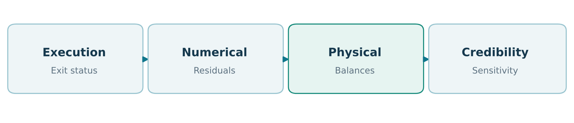
A run ending without a fatal error is not necessarily trustworthy. Keep at least four separate questions in view:
| Level | Question | Minimum evidence |
|---|---|---|
| Execution | Did the program exit correctly? | Exit status, complete log, no fatal errors |
| Numerical | Are the discrete equations solved stably? | Residuals, continuity, Courant number, no uncontrolled oscillations |
| Physical | Does the solution satisfy the problem constraints? | Balances, orders of magnitude, boundary conditions, pressure drop, flow rate |
| Credibility | Is the result overly dependent on discretisation? | Mesh, time-step, numerical scheme and model sensitivity |
Checking residuals mainly addresses the second row. Accepting the solution also requires physical observables and, ultimately, a numerical sensitivity study.
Optional background — residual versus accuracy. A residual indicates how well a discrete algebraic system is satisfied in a particular solve; a small value does not establish how accurately the discretisation represents the continuum equations. A simulation can converge to a result that is consistent with an excessively coarse mesh.
Deep dive · Verification and validation: two different questions
The reference literature on CFD credibility (for example the AIAA G-077 guide and Roache’s work) separates two activities:
- Verification: “am I solving the equations right?”. It concerns the code and the numerical solution: iterative convergence (residuals, balances), convergence with mesh and time step, estimation of discretisation error.
- Validation: “am I solving the right equations?”. It compares the result with physical reality (experiments, exact solutions of representative problems) and tests the model: laminar or turbulent, boundary conditions, fluid properties.
The “Numerical” and “Credibility” rows of the table are verification; the “Physical” row bridges towards validation. This guide covers iterative convergence and balances. Mesh convergence is the next step: in case 02 of the OpenFOAM 14 path it is carried out with a comparison against the Poiseuille solution.
2. Before running: the essential checklist
Work on a copy of the case, not the reference or an ongoing calculation. Keep 0/, constant/ and system/, and record which variant you are working on. From PowerShell:
ssh USER@SERVEROn Linux, after initialising the OpenFOAM environment:
foamVersion
cd ~/cases/myCase
pwd
ls -la
grep -E '^[[:space:]]*(solver|startFrom|endTime|deltaT|adjustTimeStep|writeControl|writeInterval)' system/controlDict
checkMesh > "log.checkMesh_$(date +%Y%m%d_%H%M%S)" 2>&1
tail -n 25 log.checkMesh_*
That final command is convenient only if the folder contains few previous logs; otherwise use the specific filename printed or recorded for the check. Look for Mesh OK, as well as any warnings about skewness, non-orthogonality, negative cell volumes, unexpected patches and strongly distorted cells. Mesh OK does not mean that the resolution is sufficient.
For incompressible cases using OpenFOAM Foundation 14, the modular solver typically runs through foamRun, with solver incompressibleFluid; in system/controlDict. Do not blindly apply old solver recipes without checking the release and case.
Before starting, check geometry and SI units, patch names in constant/polyMesh/boundary, consistency of initial fields in 0/, fvSchemes/fvSolution, available disk space and write permissions. Check the dimensions of p: in standard incompressible cases it is often kinematic pressure, not pascals.
Deep dive · Reading checkMesh: the thresholds behind the warnings
Lines starting with *** are the warnings. The main ones, with checkMesh’s default thresholds:
| Check | Warning when | What it implies |
|---|---|---|
| Non-orthogonality | angle above 70° (“severely non-orthogonal”) | the face-normal gradient needs correction; use nNonOrthogonalCorrectors and limited schemes |
| Skewness | maximum above 4 | interpolation to face centres loses accuracy |
| Aspect ratio | above 1000 | possible linear-solver difficulties |
| Volumes and determinants | negative or zero volumes, low determinant | mesh not usable: it must be fixed |
For a stricter check before a long run:
checkMesh -allGeometry -allTopology > log.checkMesh_full 2>&1
grep -n '\*\*\*' log.checkMesh_full
The meaning of non-orthogonality and skewness for schemes is developed in Part 5: fvSchemes and for correctors in Part 6: fvSolution.
Deep dive · Quick pre-launch checks from the command line
foamDictionary -entry solver system/controlDict          # solver module
foamDictionary -entry dimensions 0/p                      # [0 2 -2 0 0 0 0] = kinematic pressure
grep -E '^[[:space:]]+[A-Za-z]' constant/polyMesh/boundary | head -n 20   # patch names
df -h .                                                   # free space
touch .write_ok && rm .write_ok && echo "write OK"         # permissions
Recording the output of these commands in the assessment record of section 7 makes later variants comparable.
3. Reading the log during a run
Run from the case directory in a persistent session (tmux, where available), with a new, uniquely named log:
LOG="log.foamRun_$(date +%Y%m%d_%H%M%S)"
echo "Log: $LOG"
foamRun > "$LOG" 2>&1
printf 'Exit code: %s\n' "$?"
To monitor a run already in progress, use a second SSH session:
tail -n 50 -f log.foamRun_20261016_153000Replace the sample filename with the actual one. Ctrl+C here stops tail only, not the solver running in the other session. If you launched the solver in the foreground of the same terminal, Ctrl+C instead interrupts that solver; the distinction matters.
A typical excerpt, fabricated solely for illustration, might look like this:
Time = 120
smoothSolver: Solving for Ux, Initial residual = 0.00038, Final residual = 4.2e-07, No Iterations 3
GAMG: Solving for p, Initial residual = 0.0016, Final residual = 8.1e-06, No Iterations 5
time step continuity errors : sum local = 2.3e-07, global = -1.1e-09, cumulative = 7.0e-06
ExecutionTime = 54.12 s ClockTime = 55 s| Log term | Correct interpretation | What to investigate |
|---|---|---|
Time = ... | Simulated time or pseudo-time counter, depending on the case | Do not automatically treat this as wall-clock seconds |
Initial residual | Residual before the linear-system solve | High plateau, sustained growth or unphysical oscillation |
Final residual | Residual at the end of that particular linear solve | Does not alone prove overall convergence |
No Iterations | Linear-solver iterations for a field | Rapid increases or routinely hitting an iteration limit |
continuity errors | Local/global conservation indicators for a step | Accumulating drift or persistently high global errors |
Courant Number | Time-advection indicator where reported | Unexplained peaks; acceptable value depends on the scheme |
ExecutionTime/ClockTime | CPU time / elapsed time | Unusual slowdown or poor scaling |
Optional background — steady vs transient. In a steady case, fields and monitored observables are expected to settle. In a physically unsteady transient case, sustained oscillations can be real: judge iteration convergence per time step, balances and time-step independence, rather than demanding that residuals decrease monotonically across the entire time history.
Quick searches on Linux (when the patterns occur):
grep -nE 'FOAM FATAL|Floating point exception|nan|NaN|not converged|Courant Number|continuity errors' log.foamRun_20261016_153000 | tail -n 40
grep 'ExecutionTime' log.foamRun_20261016_153000 | tail -n 5
On Windows, download the log with FileZilla / SFTP and open it with klogg or Notepad++; to search it in PowerShell:
Select-String -Path 'C:\CFD\logs\log.foamRun_20261016_153000' -Pattern 'FOAM FATAL','Courant Number','continuity errors'A log downloaded during a run is a partial snapshot: download it again to include later steps.
Deep dive · How OpenFOAM normalises residuals
For a linear system A x = b, OpenFOAM does not report the raw norm of b − A x, which would depend on units and problem size, but a normalised residual:
r = Σ|b − A x| / ( Σ|A x − A x̄| + Σ|b − A x̄| + 10−20 )
where x̄ is the field average. The denominator measures the amplitude of variations in the field, which is why a residual of 10−3 means roughly the same thing for pressure and velocity. Two practical consequences: a nearly uniform field (small denominator) can show high residuals even with modest errors; a small “Initial residual” at the start of a transient step says the field changes little from one step to the next, not that the solution is accurate.
Tolerances, relTol and iterations are covered in Part 6.
Deep dive · Exit status, tee and pipefail
In the guide’s command the output goes straight to the file, so $? is the exit status of foamRun: 0 when the solver ended normally, non-zero after a fatal error. If you use tee to watch and save at once, $? becomes that of tee (almost always 0) and the error would be hidden. Two bash remedies:
set -o pipefail
foamRun 2>&1 | tee "$LOG"
echo "Exit code: $?"

# oppure / or
foamRun 2>&1 | tee "$LOG"; echo "Exit code: ${PIPESTATUS[0]}"
In tmux, use one window for the solver and one for tail -f and grep: Ctrl+B then C creates the second window, Ctrl+B then N switches between them.
4. Recording residuals and probes with function objects
OpenFOAM 14 ships reusable function-object configurations. Using the files from the installed release is safer than copying snippets written for another OpenFOAM distribution or vintage.
From a test case directory, run:
foamPostProcess -list | less
foamInfo residuals
foamGet residuals
foamGet probes
The foamGet commands create the corresponding files in system/ (if files already exist, back them up and check any impending overwrite first). Edit system/probes in Notepad++ and transfer with FileZilla; use coordinates inside the domain and fields present in the case. Illustrative excerpt:
fields (p U);
probeLocations
(
    (0.010 0.000 0.000)
    (0.040 0.000 0.000)
);
The coordinates are examples, not universal valid probe positions: check them against the actual domain in ParaView. Standard probes reads values from the nearest cell; select another sampling function for interpolated or sectional measurements when required.
In system/functions (create the file if missing; if present, merge with existing entries rather than replacing them), add:
#includeFunc residuals
#includeFunc probes
Depending on run settings, typical outputs include:
postProcessing/
  residuals/0/residuals.dat
  probes/0/p
  probes/0/U
The 0 subdirectory is illustrative: it can change after a restart or with startTime. Inspect with find postProcessing -maxdepth 3 -type f | sort.
If the Linux server has a graphical display and gnuplot, you can monitor residuals on the server with:
foamMonitor -l postProcessing/residuals/0/residuals.datFor a Windows-centred workflow you do not need foamMonitor: periodically download the file using FileZilla and plot it in Calc, Excel or Python. This is an option, not a mandatory dependency.
To inspect available operations without waiting for another run, check the installed options or perform post-processing of saved time directories, depending on the function object:
foamPostProcess -help
foamPostProcess -list
Not every observable can be reconstructed after the fact: if necessary underlying data were not saved, configure the monitor before running.
Deep dive · File formats and a Python script for residuals
Files under postProcessing are text with comment lines starting with #. residuals.dat has a header with column names (time and one initial residual per field, with possible N/A when a field is not solved in that step). Probe files have one comment line per probe with its coordinates; in the U file each value is a vector in brackets (Ux Uy Uz).
A script that reads the actual header instead of assuming the columns (needs Python with matplotlib on Windows):
# plot_residuals.py  -  python plot_residuals.py residuals.dat
import sys
import matplotlib.pyplot as plt

names, rows = None, []
for line in open(sys.argv[1], encoding='utf-8', errors='replace'):
    s = line.strip()
    if not s:
        continue
    if s.startswith('#'):
        tok = s.lstrip('#').split()
        if tok and tok[0] == 'Time':
            names = tok                    # last header line holding the column names
        continue
    rows.append(s.split())

for j, name in enumerate(names[1:], start=1):
    t, r = [], []
    for row in rows:
        if j < len(row) and row[j] not in ('N/A', 'nan'):
            t.append(float(row[0])); r.append(float(row[j]))
    if r:
        plt.semilogy(t, r, label=name)
plt.xlabel('Time'); plt.ylabel('Initial residual'); plt.grid(True, which='both', alpha=0.3)
plt.legend(); plt.tight_layout(); plt.savefig('residuals.png', dpi=150)
print('plot saved to residuals.png')
For the probes U file, brackets can be removed on the server before importing with sed 's/[()]//g' postProcessing/probes/0/U > U_probes.txt: each line becomes time followed by three components per probe.
Deep dive · Where the shipped configurations live
foamGet copies into the case a file taken from $FOAM_ETC/caseDicts/functions. Before using it, read its parameters with foamInfo and look at the copy:
ls $FOAM_ETC/caseDicts/functions
foamInfo probes
cat system/probes
Besides residuals and probes the same directory holds ready configurations for patch averages and flows, line sampling, forces and more. Page 7.4 Sampling and monitoring data of the v14 User Guide describes the main ones.
5. Monitor pressure drop and flow rate, not just residuals
For a channel flow problem, the operator can monitor pressure averages over inlet/outlet patches and the through-patch flow rates as the calculation advances. A suitable general OpenFOAM 14 method is surfaceFieldValue.
Add the following to system/functions, in addition to the directives above, for patches really called inlet and outlet:
pInlet
{
    type            surfaceFieldValue;
    libs            ("libfieldFunctionObjects.so");
    patch           inlet;
    operation       areaAverage;
    writeFields     false;
    fields          (p);
    writeControl    timeStep;
    writeInterval   1;
}

pOutlet
{
    type            surfaceFieldValue;
    libs            ("libfieldFunctionObjects.so");
    patch           outlet;
    operation       areaAverage;
    writeFields     false;
    fields          (p);
    writeControl    timeStep;
    writeInterval   1;
}

qInlet
{
    type            surfaceFieldValue;
    libs            ("libfieldFunctionObjects.so");
    patch           inlet;
    operation       sum;
    writeFields     false;
    fields          (phi);
    writeControl    timeStep;
    writeInterval   1;
}

qOutlet
{
    type            surfaceFieldValue;
    libs            ("libfieldFunctionObjects.so");
    patch           outlet;
    operation       sum;
    writeFields     false;
    fields          (phi);
    writeControl    timeStep;
    writeInterval   1;
}
The patch must exist, and p and phi must be available in the case. Output series will be under postProcessing/pInlet/..., pOutlet/..., qInlet/... and qOutlet/...; inspect actual filenames and column headers before analysis. This is OpenFOAM Foundation v14 syntax, not the sometimes different regionType/name syntax of other distributions.
Calculations after exporting the series:
- Mean pressure difference:
Δp = p_mean,in − p_mean,out. - For a standard incompressible solver with kinematic
p, dimensions[0 2 -2 0 0 0 0]:ΔP [Pa] = ρ [kg/m³] × Δp [m²/s²], for constant density. - If
palready has dimensions of pressure in Pa, do not multiply by density. - For volumetric
phi,Q_inis usually negative since the patch normal points outward, whereasQ_outis positive. With mass-fluxphi, units are kg/s: verify the field dimensions. - With one inlet and one outlet, relative imbalance:
ε_Q = |Q_in + Q_out| / ((|Q_in|+|Q_out|)/2) × 100%. For additional open patches, include all fluid boundaries.
Purely illustrative calculation: p_in − p_out = 6.2 m²/s², ρ = 1000 kg/m³ → ΔP = 6200 Pa; Q_in = −2.500×10⁻⁴ m³/s, Q_out = +2.495×10⁻⁴ m³/s → ε_Q ≈ 0.20%. These values are not acceptance thresholds.
Optional background — which pressure? When comparing with an instrument, define matching sections and distinguish static pressure, hydraulic pressure difference, total head and local losses. Area-averaged pressures at an inlet and outlet do not always equal the irreversible pressure loss: acceleration, nonuniform velocity profiles and elevation may matter.
Deep dive · An order-of-magnitude check on the path’s channel
In the trainingChannel of Part 3 (10 × 5 mm cross-section, uniform inlet velocity 0.05 m/s) the expected flow rate is Q = U · A = 0.05 × 5.0×10⁻⁵ = 2.5×10⁻⁶ m³/s. qInlet should therefore be close to −2.5×10⁻⁶ from the first step, because the boundary condition imposes it, while qOutlet tends to +2.5×10⁻⁶ as the field settles.
For the pressure drop between two parallel plates at distance H in developed laminar flow, Δp_kin = 12 ν L U_mean / H² (kinematic pressure): this is the relation used in case 01 for the Poiseuille validation. In a rectangular duct the coefficient changes with the aspect ratio, but the order of magnitude remains a useful check before looking at the decimals.
Deep dive · Ready-made alternatives: patchAverage and patchFlowRate
The configurations shipped with OpenFOAM 14 include functions already set up for patch averages and flow rates, callable with arguments on one line of system/functions. Before using them, read the parameters your installation accepts:
foamInfo patchAverage
foamInfo patchFlowRate
With the parameters confirmed by foamInfo, the form is like:
#includeFunc patchAverage(patch=inlet, fields=(p))
#includeFunc patchAverage(patch=outlet, fields=(p))
#includeFunc patchFlowRate(patch=inlet)
#includeFunc patchFlowRate(patch=outlet)
The result is equivalent to the four explicit blocks; the guide’s blocks remain preferable when you want to see and control every option (operation, writeControl, writeInterval).
Automatic stopping does not mean physical validation
Some steady-state cases use SIMPLE/residualControl in system/fvSolution to specify automatic stopping criteria. Inspect the local configuration:
grep -n -A 14 'residualControl' system/fvSolutionA solver convergence message means the configured stopping conditions were met: it does not replace pressure, flow balance or discretisation checks. In transient cases, iteration and stopping rules have different meanings.
Deep dive · What residualControl looks like
SIMPLE
{
    nNonOrthogonalCorrectors 0;

    residualControl
    {
        p               1e-2;
        U               1e-3;
        "(k|epsilon|omega)" 1e-3;
    }
}
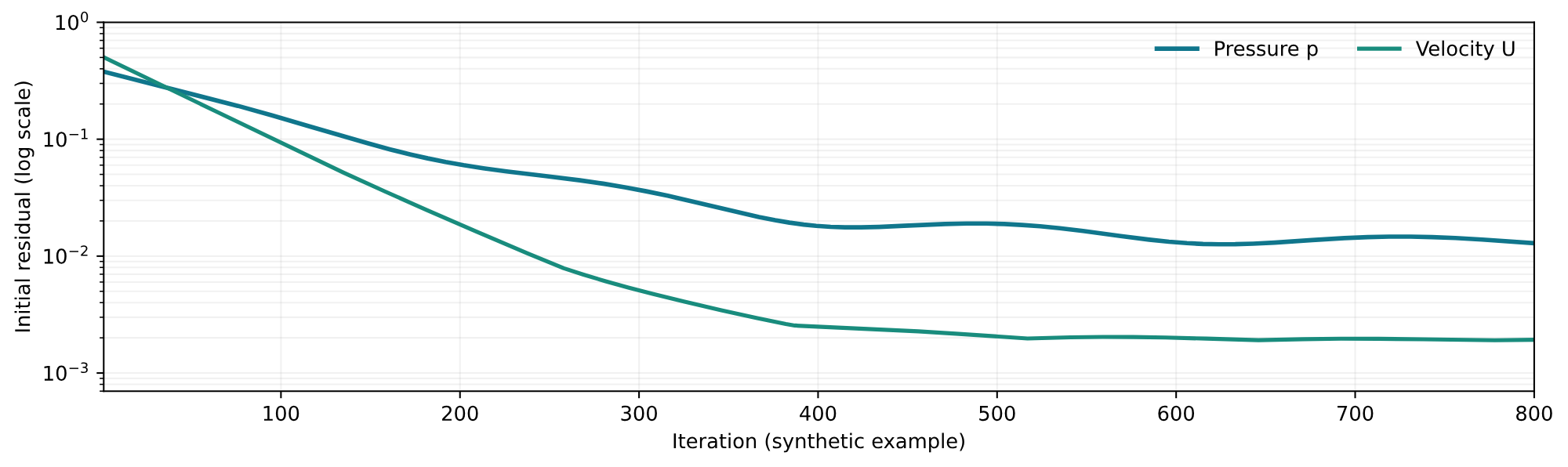
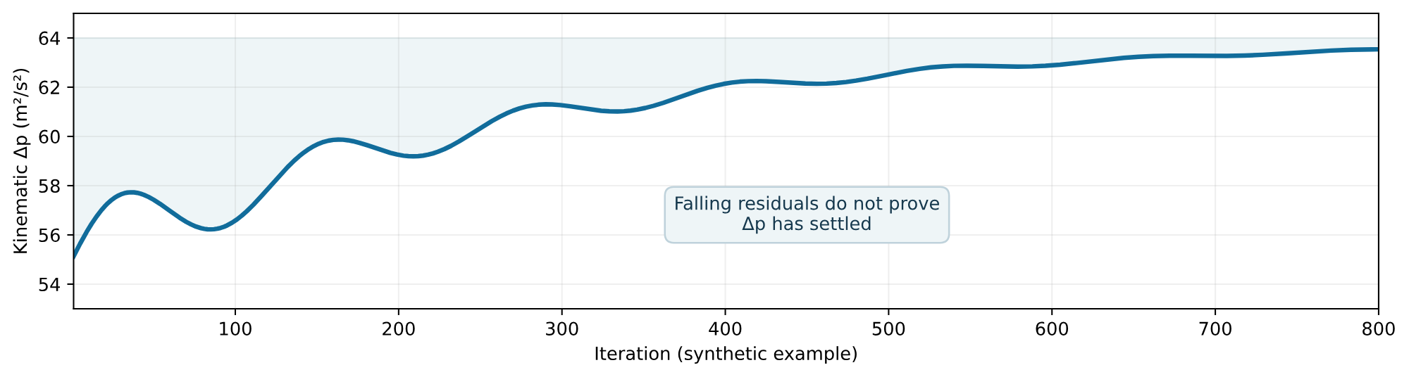
Each value is the threshold on the field’s Initial residual: when every listed field falls below its threshold in the same iteration, the solver writes the last time and exits with a message like SIMPLE solution converged in ... iterations. The thresholds are not universal: with loose values the run can stop while Δp is still changing. That is why the guide asks you to compare the stop with the observables of figure 3. The SIMPLE and PIMPLE algorithms are explained in Part 6.
6. Recognising three common patterns
| Observation | Possible interpretation | First controlled response |
|---|---|---|
Residuals decrease but Δp still drifts | Local algebraic convergence, global observable not settled | Continue monitoring and assess Δp stability over a stated window |
| Residuals and continuity errors grow; Courant peaks | Numerical instability, unsuitable initial/BC setup or time step | Recheck BCs, mesh, time step; compare with baseline |
Low residuals and stable Δp, but poor balance | Missing patches, incorrect fluxes, setup/calculation problems | Identify all open patches, account for Σphi and volume sources |
Severe warning from checkMesh | Geometry/discretisation problem | Fix and recheck mesh rather than random solver tolerance changes |
FOAM FATAL ERROR or Floating point exception | Abnormal termination, no valid result | Keep log/configuration; identify the first underlying causal message |
Oscillations do not automatically indicate an error: they may be physical in transient flows. The right response depends on the model and its goals. Do not change mesh, schemes, relaxation and boundary conditions all at once: doing so obscures the cause.
Debugging rule: retain a baseline, change one factor at a time, create a new log and compare a consistent set of metrics.
Deep dive · Finding the first causal message and comparing two variants
In a log that ends with an error, the last message is often a consequence. Find the first occurrence and read the lines before it:
grep -n -m1 -E 'FOAM FATAL|Floating point exception|nan' log.foamRun_20261016_153000
sed -n '1180,1240p' log.foamRun_20261016_153000      # intervallo attorno alla riga trovata / range around the line found
With two copies of the case (baseline and variant), the dictionary diff shows exactly what changed:
diff -ru myCase_v01/system myCase_v02/system
diff -ru myCase_v01/constant/momentumTransport myCase_v02/constant/momentumTransport
diff -ru myCase_v01/0 myCase_v02/0
If the diff shows more than one changed factor, comparing the two logs cannot attribute the cause.
7. Worked exercise: a reproducible assessment
The exercise uses any already verified incompressible-flow case with patches named inlet/outlet; adapt the names if necessary. No new geometry is required to make use of the guide.
- Duplicate the case into a new folder such as
myCase_monitor_v01; do not delete the earlier version’s data. - Run
checkMeshand keep the timestamped output. - Create
system/residualsandsystem/probesusingfoamGet, checking whether files already exist. - Create or merge
system/functions; add pressure/flow-rate monitors from chapter 5 only after checking patch names. - Start
foamRunintmuxor another persistent session, and record the exact new log filename. - In a second session, watch
tail -f ...; look for errors, continuity data, Courant (where relevant), and execution times. - Download only
log.*andpostProcessing/with FileZilla. Full CFD field volumes are normally unnecessary for convergence plots. - On Windows, view the log in klogg; import
.dat,p, andUseries into LibreOffice Calc, Excel or Python, respecting comment/header formats. - Produce at least three graphs: residuals (log y-axis when useful),
ΔporΔPagainst iteration/time, and flow imbalanceε_Qagainst iteration/time. - Report the final window analysed, sample count and
Δpvariation within it, for example max–min relative to its nonzero mean. Clearly identify steady or transient runs.
Teaching pitfall. If residuals seem to have plateaued but Δp has changed by 5% over the last observation window, stability of the quantity of interest has not yet been demonstrated. Conversely, if residuals fall by another two orders of magnitude with no change in Δp, prioritise conservation and discretisation sensitivity checks. 5% is an example, not a universal cut-off.
Deep dive · A script for Δp, ε_Q and the settling window
The script reads the four series downloaded with FileZilla (the postProcessing folder copied to Windows), computes Δp and ε_Q step by step and summarises the last N rows: mean, relative variation (max−min)/|mean| and slope. It uses only the Python standard library.
# monitor_report.py  -  python monitor_report.py <downloaded postProcessing folder> [N]
import sys, re, pathlib, statistics as st

def read_series(path):
    # returns (times, values) reading the first column after time; skips '#' comments
    t, v = [], []
    for line in open(path, encoding='utf-8', errors='replace'):
        if not line.strip() or line.lstrip().startswith('#'):
            continue
        tok = line.split()
        try:
            t.append(float(tok[0])); v.append(float(tok[1]))
        except (ValueError, IndexError):
            pass
    return t, v

def find(root, name):
    files = sorted(pathlib.Path(root, name).rglob('*.dat'))
    if not files:
        sys.exit('no .dat file in ' + str(pathlib.Path(root, name)))
    return files[-1]          # the latest start subfolder (restart)

root = sys.argv[1]
N = int(sys.argv[2]) if len(sys.argv) > 2 else 100
series = {k: read_series(find(root, k)) for k in ('pInlet', 'pOutlet', 'qInlet', 'qOutlet')}
n = min(len(s[1]) for s in series.values())
pin, pout = series['pInlet'][1][:n], series['pOutlet'][1][:n]
qin, qout = series['qInlet'][1][:n], series['qOutlet'][1][:n]
t = series['pInlet'][0][:n]
dp = [a - b for a, b in zip(pin, pout)]
eps = [abs(a + b) / ((abs(a) + abs(b)) / 2) * 100 for a, b in zip(qin, qout)]
w = slice(max(0, n - N), n)
dpw, epw, tw = dp[w], eps[w], t[w]
m = st.mean(dpw)
slope = (dpw[-1] - dpw[0]) / (tw[-1] - tw[0]) if tw[-1] != tw[0] else 0.0
print(f'total samples {n}, final window {len(dpw)} samples, from t={tw[0]} to t={tw[-1]}')
print(f'mean dp {m:.6g}   (max-min)/|mean| = {(max(dpw)-min(dpw))/abs(m)*100:.3g} %   slope {slope:.3g} per unit time')
print(f'mean eps_Q {st.mean(epw):.3g} %   max {max(epw):.3g} %   Q_in {st.mean(qin[w]):.6g}   Q_out {st.mean(qout[w]):.6g}')
with open('monitor_report.csv', 'w') as f:
    f.write('time,dp,eps_Q_percent\n')
    for a, b, e in zip(t, dp, eps):
        f.write(f'{a},{b},{e}\n')
print('full series written to monitor_report.csv')
Usage: python monitor_report.py C:\CFD\logs\myCase\postProcessing 200. The slope multiplied by the window length tells how much Δp is still changing: if it is of the same order as the variation you accept, the window has not settled yet. monitor_report.csv opens directly in Excel or Calc for plotting.
Assessment record to attach to every simulation
| Parameter or check | What to record |
|---|---|
| Case identifier and dictionary revision | Name, date, location, notes |
| OpenFOAM version and model | foamVersion, solver, physical regime |
| Mesh | Cell count, checkMesh results, changes |
| Time and numerical discretisation | deltaT/maxCo, fvSchemes, fvSolution |
| Execution status | Completed/interrupted, exit code, log filename |
| Numerical indicators | Residuals, continuity, Courant (if applicable) |
| Physical quantities | Δp / ΔP, Q_in, Q_out, ε_Q and units |
| Settling assessment | Selected window, means, variation |
| Further validation | Theory/experiment and mesh/time-step studies |
8. Common mistakes when analysing from Windows
Mistake: a .dat file is empty or contains just a header. The solver may not have written a valid sample yet. Check writeControl/writeInterval, warnings in the solver log, and the appropriate restart folder under postProcessing.
Mistake: FileZilla appears to show old data. A local file is a static download: re-download and check size and modification time. Editing a local dictionary does not update a running remote case until explicitly transferred.
Mistake: charts imported into Excel make no sense. Data often contain # comment lines, whitespace separators and vector values like (Ux Uy Uz). Use appropriate delimited-text import settings, or split and normalise vector components first. Do not assume the U file is a plain four-column table.
Mistake: p is always interpreted as Pa. Read the field file, for example 0/p, and inspect dimensions: [0 2 -2 0 0 0 0] denotes kinematic pressure; [1 -1 -2 0 0 0 0] is pressure in pascals.
Mistake: low ε_Q is treated as sufficient proof. A good global balance cannot exclude unresolved local flow structures, wall effects, wrong velocity distributions or an under-resolved mesh.
Mistake: a universal threshold is applied to every simulation. Residuals, Courant limits and settling must be related to the simulation goals and physical regime. Document your criteria before interpreting results.
Deep dive · Importing into Excel with non-English regional settings
OpenFOAM writes numbers with a decimal point (2.5e-06). Excel set to a locale that uses a decimal comma (Italian, German, French…) misreads them: opened with a double click, many values become text or dates. The correct procedure:
- Data → From Text/CSV, choose the file;
- file origin: UTF-8; delimiter: Space, with “treat consecutive delimiters as one”;
- in Transform Data (Power Query) remove the rows starting with
#; - change the column types with Using Locale → English (United States), so the point is read as decimal separator.
In LibreOffice Calc: Language → English (USA) in the text import dialog, space separator, “Merge delimiters”. The monitor_report.py script of section 7 avoids the issue by writing a CSV with commas as field separators and points as decimal separators, to be imported with the same setting.
9. Final checklist and references
Before calling a result reliable: check that no fatal error occurred, that the mesh is suitable, field and BC units are coherent, residuals and numerical indicators are appropriate, balances are satisfactory, quantities of interest have stabilised in the physically relevant sense, and discretisation effects have been considered.
Primary technical references (OpenFOAM Foundation 14):
- OpenFOAM v14 — User Guide — general structure, modular solvers, tutorials.
- 7.4 — Sampling and monitoring data —
foamGet,probes,residuals,foamMonitor. - 2.1 — Backward-facing step — execution, log and stopping criteria in a steady example.
- v14 API — surfaceFieldValue —
patchsyntax andsum/areaAverageoperations. - v14 API — Function objects —
system/functionsand execution/write controls. - 7.3 — Post-processing functionality — feature list and dimensional context.
- klogg — optional Windows tool for searching large logs.
Plots are schematic and use synthetic teaching data, not measured CFD results. Dictionary snippets must be adapted to each case’s patch names, fields and geometry.
Further useful references
- klogg — optional Windows viewer for large logs.
Related guides: OpenFOAM on a Linux server, working from Windows (transfers, SSH, tmux, ParaView) and the Learning OpenFOAM 14 path, in particular controlDict and fvSolution.