

OpenFOAM 14 Part 5: fvSchemes, from Equations to Discretisation
Part 5 of 8 of the case-building series in Learning OpenFOAM 14. Part 4 explained how system/controlDict selects the solver module, advances time and writes results; this part opens system/fvSchemes, the dictionary that tells OpenFOAM how to turn each term of the equations into a discrete finite-volume approximation.
The numerics behind the dictionary. The subject is the path from the terms of the partial differential equations (time, gradient, advection, diffusion) to the fvSchemes entries (ddt, grad, div, laplacian, snGrad), and from these to the actual discretisation: face values, fluxes and cell equations. Each “Deep dive” box expands a point with the finite-volume mathematics, how OpenFOAM 14 implements it, the alternatives, the typical errors and the practical checks.
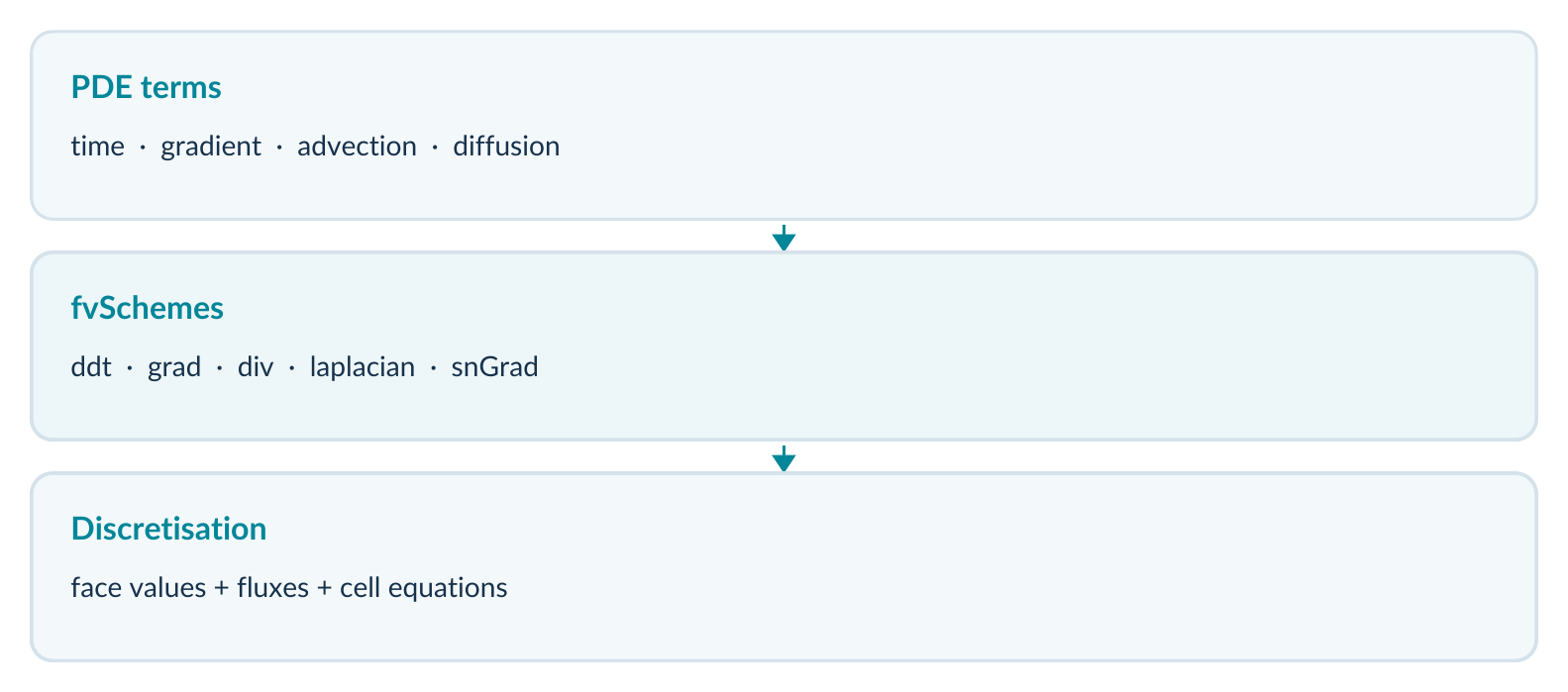
fvSchemes entries (ddt, grad, div, laplacian, snGrad), which produce the discretisation: face values, fluxes and cell equations.How to use this part
Prerequisites. This part assumes the first seven CFD exercises of the series (starting from the laminar channel flow and Poiseuille validation) and the preceding units: Part 1 (case anatomy and dictionary language), Part 2 (meshing with blockMeshDict), Part 3 (fields and boundary conditions) and Part 4 (controlDict). It reuses the three-dimensional laminar channel with the patches inlet, outlet and walls.
Scope. OpenFOAM Foundation 14. Read and modify system/fvSchemes, interpret its entries, compare numerical choices and troubleshoot configuration errors.
Reading path
Main track: PDE terms → dictionary anatomy → time, gradient and divergence schemes → Laplacian and surface-normal gradients → controlled experiments. The Optional refresher boxes can be skipped by experienced CFD readers.
Reference guide: OpenFOAM v14 User Guide, §4.5 — Numerical schemes. The deep-dive boxes are closed by default: click the title to open one.
Before you begin: learning contract
The aim is configuration literacy, not to memorise every numerical method. By the end, you should be able to read a new entry, connect it to an equation term, and locate the official v14 documentation that defines its use.
Prerequisites
- OpenFOAM Foundation 14 is enabled in the shell:
foamVersion. - You have an independent copy of the channel case from Parts 2–4; do not edit the teaching master.
- You can read
0/U,0/p,system/controlDict, and a basicblockMeshDict. - You know that the solver module must be compatible with the mesh, fields and physical properties.
What you will be able to do
- Map a term in the governing equations to an
fvSchemessub-dictionary. - Explain what
Euler,Gauss linear,upwind,linearUpwindandcorrectedare doing. - Distinguish a global
defaultfrom an explicit per-term override. - Compare two schemes by changing one controlled parameter in copied cases.
- Use
foamSearchandfoamDictionaryto inspect authentic v14 configurations.
Optional refresher · Why discretise?
A continuous PDE describes variations at arbitrarily many spatial points. A finite-volume calculation instead stores values in cells and evaluates fluxes across a finite set of faces. Discretisation is the construction of those discrete approximations.
Deep dive · From PDE to algebraic system: what discretisation actually produces
The finite-volume method starts from the integral form of the conservation equations. The equation is integrated over each cell (control volume) VP and Gauss’s (divergence) theorem turns the volume integrals of divergences into surface integrals, i.e. into sums over the faces of the cell. For the generic quantity a of the transport equation in section 2:
∫V ∂a/∂t dV  +  ∮S (U a)·dS  =  ∮S (Γ ∇a)·dS  +  ∫V S dV

(∂a/∂t)_P V_P  +  Σ_f F_f a_f  =  Σ_f Γ_f |S_f| (∇a)_f·n_f  +  S_P V_P
Here Ff = Sf·Uf is the volumetric flux through face f (the phi field), af is the value of the quantity on the face, Γf the diffusion coefficient interpolated to the face and (∇a)f·nf the face-normal gradient. Each of these ingredients needs an approximation rule: that is exactly what fvSchemes chooses. Once every af and every face gradient are written as a combination of the cell-centre values of neighbouring cells, the equation of each cell becomes a linear relation:
a_P · a_P_value + Σ_N a_N · a_N_value = b_Pwith a diagonal coefficient aP, one coefficient aN for each neighbouring cell sharing a face, and a source bP that collects sources, explicit contributions and boundary values. Assembling all cells gives a sparse matrix: on a hexahedral mesh each row has at most 7 non-zero entries (the cell and its 6 neighbours). fvSchemes decides how the coefficients are built; fvSolution (Part 6) decides how the resulting system is solved. In the source code the distinction shows up as two namespaces: fvm:: (finite volume method) produces implicit matrix contributions, fvc:: (finite volume calculus) evaluates a term explicitly from the current values; both read their scheme from the same fvSchemes sub-dictionary.
Rule for the entire part
Use the numerical choices as teaching examples, not as recommended defaults for the catalyst reactor or any unrelated geometry.
Deep dive · How to find the v14 documentation that defines an entry
The goal “locate the official v14 documentation” has three concrete tools, all available in an OpenFOAM 14 shell. The first is section 4.5 of the v14 User Guide, organised by sub-dictionary (4.5.1 time schemes, 4.5.2 gradients, 4.5.3 divergences, 4.5.4 surface-normal gradients, 4.5.5 Laplacians, 4.5.6 interpolation). The second is the set of installed tutorials in $FOAM_TUTORIALS, which show how the developers use the schemes on real cases: foamSearch extracts the value of one entry from every file with a given name and prints the sorted list without duplicates; with the -count option (see foamSearch -help) it also prints how many times each value occurs. The third is foamToC, which lists the run-time selectable classes compiled into the installation: if a scheme name does not appear, it is not available in your version.
# Which scheme names are actually used, and how often, in the v14 tutorials
foamSearch -count "$FOAM_TUTORIALS" fvSchemes "divSchemes/div(phi,U)"

# Which tutorials use a given keyword (plain grep over the installed tree)
grep -rl "linearUpwind" "$FOAM_TUTORIALS"/incompressibleFluid/*/system/fvSchemes

# Which run-time selectable classes contain a name (v14 table-of-contents tool)
foamToC -search linearUpwind
There is also an “experimental” and completely safe way, to be used only in a copy of the case: write a non-existent name on purpose (for example div(phi,U) Gauss xyz;). At start-up OpenFOAM stops with an error of the form “Unknown discretisation scheme xyz” followed by a Valid schemes are list: that is the authentic list of schemes compiled for that operator and field type. It is the final arbiter: what your executable accepts, not what a web page about another OpenFOAM branch says.
1. Where fvSchemes belongs
The dictionary system/fvSchemes assigns numerical approximations to the differential operators assembled by the selected OpenFOAM module. It does not specify the physical viscosity, velocity boundary values or the linear solver convergence tolerance.
| Case layer | Typical responsibility |
|---|---|
0/ | Field initial values and patch boundary conditions. |
constant/ | Mesh and physical properties/models. |
system/controlDict | Time, writing, run configuration and solver-module selection. |
system/fvSchemes | Discretisation of derivatives, fluxes and interpolation. |
system/fvSolution | Linear solvers, tolerances and pressure–velocity algorithm controls. |
Two different numerical questions
Conceptual contrast:
fvSchemes:     div(phi,U)   Gauss linearUpwind grad(U);
fvSolution:    p solver settings, tolerances, correctors
The first entry answers how the advection term is approximated. The second set of controls answers how the discretised algebraic system is solved. This distinction is the central bridge from this part to Part 6.
Version 14 note
The reference workflow uses the incompressibleFluid solver module through foamRun, as introduced in Part 4. The numerical operator names in fvSchemes depend on the equations and models active in that module.
Deep dive · When and how foamRun reads fvSchemes
fvSchemes is not read “all at once” like a generic configuration module. At start-up, foamRun reads controlDict, loads the module named by solver, and constructs the mesh and fields; the fvSchemes dictionary is opened together with the mesh, but each individual entry is looked up only when an operator requests it, i.e. when the module first assembles the corresponding term. Two practical consequences: an error about a missing entry can appear after several normal-looking log lines (when the first equation is built, not when the file is read); and an entry that is written but never requested produces neither errors nor effects.
The dictionary is registered as modifiable at run time: OpenFOAM checks during the run whether the system/ dictionaries have been modified (a global behaviour, governed by the system controlDict under $FOAM_ETC); if you save a change to fvSchemes while the run is going, the file is re-read at the start of a later step and the log reports the re-read. This is handy for experiments but breaks traceability: in a controlled comparison (section 15) you never edit a running case. In multi-region cases each region has its own file, system/<region>/fvSchemes.
A quick check that the file is syntactically valid, without starting the solver, is to ask foamDictionary to print it in full: foamDictionary system/fvSchemes. If a brace or semicolon is missing, the error appears immediately with the line number; if the file prints, the syntax is correct (the correctness of the scheme names, however, is only discovered when the module starts).
Deep dive · The operators of the incompressibleFluid module, one by one
For the laminar channel the incompressibleFluid module solves the momentum equation and an equation for the (kinematic, p/ρ, as seen in Part 3) pressure. In continuous form the momentum equation reads:
∂U/∂t + ∇·(U U) − ∇·[ν_eff (∇U + (∇U)^T − (2/3)(∇·U) I)] = −∇pThe viscous term is split into two parts: an implicit Laplacian ∇·(νeff∇U), which holds the dominant part and goes into the matrix, and an explicit divergence of the remainder, ∇·[νeff dev2((∇U)T)], where dev2(A) = A − (2/3) tr(A) I. For an incompressible fluid the second part is almost zero, but the module assembles it anyway. Here is how the terms become operator names and which fvSchemes entry serves them, with the teaching dictionary of section 3:
// incompressibleFluid, laminar: momentum-equation operators and their names
ddt(U)                              -> ddtSchemes/default
div(phi,U)                          -> divSchemes/div(phi,U)
laplacian(nuEff,U)                  -> laplacianSchemes/default
div((nuEff*dev2(T(grad(U)))))       -> divSchemes/div((nuEff*dev2(T(grad(U)))))
grad(p)                             -> gradSchemes/default
grad(U)  (needed by linearUpwind)   -> gradSchemes/default or gradSchemes/grad(U)
In the laminar regime νeff equals the viscosity ν from constant/physicalProperties (Part 7), but the operator name stays nuEff because the momentum transport model builds it. The pressure equation adds a Laplacian of p (served by laplacianSchemes/default), face interpolations (served by interpolationSchemes/default) and normal gradients (served by snGradSchemes/default). The divergence of the face fluxes in the continuity equation, on the other hand, needs no entry: the divergence of a field already defined on faces is a plain sum, with no interpolation to choose. That is why a laminar incompressibleFluid case runs with only two explicit entries in divSchemes.
2. From an equation to six scheme families
Consider a generic transport equation. Its physical terms are discretised by different methods, even when they appear together in the same PDE.
Schematic transport equation · a is a generic transported quantity:
d(a)/dt + div(U a) = div(Gamma grad(a)) + S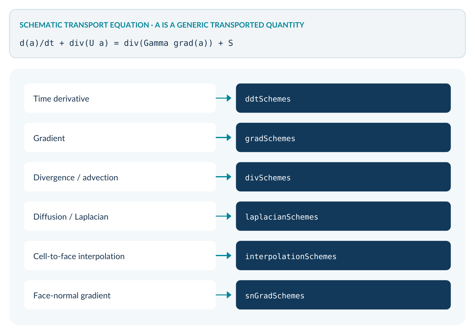
system/fvSchemes.| Operation | Sub-dictionary |
|---|---|
| Time derivative | ddtSchemes |
| Gradient | gradSchemes |
| Divergence / advection | divSchemes |
| Diffusion / Laplacian | laplacianSchemes |
| Cell-to-face interpolation | interpolationSchemes |
| Face-normal gradient | snGradSchemes |
Optional refresher · Conservation
For a cell, a flux through one face is the neighbouring cell’s opposite flux. Finite-volume face summation is therefore naturally suited to discrete conservation when fluxes are assembled consistently.
Important: a particular operator is requested only when the active equations use it. Not every case needs every explicitly named term; default entries cover many operations.
Deep dive · Discrete conservation in a numerical example
Take three cells in a row, 1 – 2 – 3, with internal faces A (between 1 and 2) and B (between 2 and 3), an inlet face to the left of cell 1 and an outlet face to the right of cell 3. In OpenFOAM each internal face belongs to an owner cell (the lower index) and a neighbour cell; the area vector Sf points from owner to neighbour, and the face flux phi is a single number stored once. When summing around the owner it enters with a + sign, around the neighbour with a − sign. Assume phiin = 2.5 × 10⁻⁶ m³/s (the channel flow rate at 0.05 m/s), phiA = 2.5 × 10⁻⁶, phiB = 2.5 × 10⁻⁶, phiout = 2.5 × 10⁻⁶ m³/s.
The net outflow of each cell is: cell 1, phiA − phiin = 0; cell 2, phiB − phiA = 0; cell 3, phiout − phiB = 0. Summing the three cells, the internal fluxes A and B appear once with + and once with − and cancel (a “telescoping sum”): what remains is phiout − phiin. That is discrete conservation: what the domain gains or loses depends only on the boundary fluxes, whatever scheme is chosen to compute face values, provided each face has one single flux value. With a finite-difference method on an unstructured grid this property is not automatic.
Conservation does not mean accuracy: even a very diffusive scheme such as upwind is perfectly conservative. The choices in fvSchemes change which value is assigned to the face, not the fact that both cells use the same value.
Deep dive · The source term S and the terms fvSchemes does not govern
In figure 2 the source term S has no sub-dictionary. A source is a volume term, not a derivative: in discrete form it simply becomes SPVP, with no interpolation needed. In OpenFOAM 14 additional sources (imposed body forces, mass or heat sources, porous zones) are defined in constant/fvModels, and constraints (velocity or temperature limits, for example) in system/fvConstraints. A source that depends on the variable itself is usually linearised as S = Su + Sp·a: the Sp part (if negative) goes on the matrix diagonal and improves stability, the Su part goes into the right-hand side.
The pressure gradient in the momentum equation, although it is a derivative, also does not appear “by name” in the generic equation: it is a gradient like any other and uses gradSchemes (in practice, within the pressure–velocity algorithm, the part that matters is the face gradient, consistent with the pressure Laplacian). Remember this when reading logs: the fact that a term is missing from the figure does not mean it has no scheme.
3. A complete teaching fvSchemes
The following compact file is a transient v14-oriented example, modelled on the operator names found in Foundation 14 incompressibleFluid tutorials. It assumes a compatible case and model set. It is not a stand-alone runnable case.
system/fvSchemes · educational transient baseline:
FoamFile
{
    format      ascii;
    class       dictionary;
    location    "system";
    object      fvSchemes;
}
ddtSchemes
{
    default     Euler;
}
gradSchemes
{
    default     Gauss linear;
}
divSchemes
{
    default     none;
    div(phi,U)  Gauss linearUpwind grad(U);
    div((nuEff*dev2(T(grad(U))))) Gauss linear;
}
laplacianSchemes
{
    default     Gauss linear corrected;
}
interpolationSchemes
{
    default     linear;
}
snGradSchemes
{
    default     corrected;
}
The additional stress-divergence entry is easy to overlook: not all terms in divSchemes are convection terms. The exact expression requested comes from the equations assembled in the module.
Deep dive · The file read line by line
| Entry | What it serves in the channel | Where it is explained |
|---|---|---|
FoamFile | Header: format, class dictionary, location system and object name. In v14 the version entry is not required. | Part 1 |
ddtSchemes/default Euler | The time derivative ∂U/∂t of the momentum equation. | Section 5 |
gradSchemes/default Gauss linear | grad(p), grad(U) requested by linearUpwind and by the viscous stress. | Sections 6–7 |
divSchemes/default none | No fallback: every divergence must be named. | Section 4 |
div(phi,U) | Advection of momentum. | Sections 8–10 |
div((nuEff*dev2(T(grad(U))))) | Explicit part of the viscous-stress divergence. | Section 8 |
laplacianSchemes/default | laplacian(nuEff,U) and the pressure Laplacian. | Section 11 |
interpolationSchemes/default | Generic cell-to-face interpolations, for example when building fluxes. | Section 13 |
snGradSchemes/default | Face-normal gradients, for example in the flux correction. | Section 12 |
For comparison with a real file, here is the content (without the header) of OpenFOAM-14 tutorials/incompressibleFluid/airFoil2D/system/fvSchemes, one of the two examples cited in the appendix. It is a steady case with the Spalart–Allmaras turbulence model: note steadyState, the bounded prefix, a second advection entry for the turbulence variable nuTilda and the wallDist sub-dictionary, required by the model.
ddtSchemes
{
    default         steadyState;
}

gradSchemes
{
    default         Gauss linear;
}

divSchemes
{
    default         none;

    div(phi,U)      bounded Gauss linearUpwind grad(U);
    div(phi,nuTilda) bounded Gauss linearUpwind grad(nuTilda);
    div((nuEff*dev2(T(grad(U))))) Gauss linear;
}

laplacianSchemes
{
    default         Gauss linear corrected;
}

interpolationSchemes
{
    default         linear;
}

snGradSchemes
{
    default         corrected;
}

wallDist
{
    method          meshWave;
}
The differences from the teaching file can all be explained by the active equations: the steady regime changes ddtSchemes and motivates bounded (section 10), the turbulence model adds a transport equation (hence one more divergence) and wall distance (hence wallDist, section 13). The rest is identical.
Deep dive · Checking what OpenFOAM reads, not what we think we wrote
OpenFOAM dictionaries can contain macros ($name), #include directives and keys written as regular expressions. The file seen in the editor can therefore differ from what the program interprets. foamDictionary shows the interpreted version:
foamDictionary -expand system/fvSchemes                    # whole file, macros and #include resolved
foamDictionary -keywords -entry divSchemes system/fvSchemes  # only the keywords of one sub-dictionary
foamDictionary -entry "divSchemes/div(phi,U)" -value system/fvSchemes
The quotes around divSchemes/div(phi,U) are required: brackets have a special meaning to the shell. The expected result of the last command, with the teaching file, is the single line Gauss linearUpwind grad(U). If an error like “keyword … is undefined” appears instead, the entry does not exist under that exact name: often because of an extra space, as in div(phi, U), which is a different key for OpenFOAM.
4. Defaults, overrides and missing terms
A default entry applies to operators in its family unless a more specific entry overrides it. The keyword none disables the generic fallback, making explicitly named terms necessary when requested by the solver.
Two lookup behaviours:
gradSchemes
{
    default Gauss linear;
    grad(U) cellLimited Gauss linear 1;
}
divSchemes
{
    default none;
    div(phi,U) Gauss upwind;
}| Question | Answer |
|---|---|
Which scheme for grad(p)? | Gauss linear, inherited from gradSchemes/default. |
Which scheme for grad(U)? | cellLimited Gauss linear 1, explicit override. |
Which scheme for div(phi,U)? | Gauss upwind, explicitly assigned. |
| What if another divergence is needed? | With divSchemes/default none, OpenFOAM needs its own matching specification. |
Why divSchemes often uses none
A divergence may describe advection or the divergence of a stress expression. Assigning one broad scheme to all divergences can conceal inappropriate treatment. Foundation v14 tutorials commonly use explicit divergence terms.
Read the dictionary structurally
An expression such as div(phi,U) is a dictionary keyword naming an operator. The expression following it, such as Gauss upwind, defines the numerical approximation. Do not read the entry as an algebraic equation.
Deep dive · The lookup algorithm, step by step
When the module builds an operator, it generates a string with its name from the names of the fields involved: fvm::div(phi, U) produces div(phi,U), fvc::grad(p) produces grad(p), fvm::laplacian(nuEff, U) produces laplacian(nuEff,U). It then looks up that string in the family’s sub-dictionary:
- if an identical key exists (or a regular-expression key that matches it), it uses that value;
- otherwise, if
defaultexists with a value other thannone, it uses the default; - otherwise (default missing or
none) it stops with a fatal input error naming the key it looked for and the dictionary it searched.
The comparison is literal: div(phi,U) and div(phi, U) are different keys, as are grad(U) and grad(u). The typical error message, for a missing divergence with default none, has this form (paths and line numbers depend on the case):
--> FOAM FATAL IO ERROR:
keyword div((nuEff*dev2(T(grad(U))))) is undefined in dictionary ".../system/fvSchemes/divSchemes"

file: .../system/fvSchemes/divSchemes from line 32 to line 36.
The message is the most reliable evidence of which operator the module actually requests: copy the key from the log into the file and assign it a suitable scheme.
Deep dive · Macros and regular expressions in v14 tutorials
With default none the files of turbulent cases would become long and repetitive. The Foundation tutorials use two tools of the dictionary language (Part 1) to avoid this. The first is the macro: define an entry with any name and recall it with $. The second is the regular-expression key, written in quotes, which applies to every name it matches. An example of the typical pattern:
divSchemes
{
    default         none;
    div(phi,U)      bounded Gauss linearUpwind grad(U);
    turbulence      bounded Gauss limitedLinear 1;
    div(phi,k)      $turbulence;
    div(phi,omega)  $turbulence;
    "div\(phi,(k|epsilon)\)"  bounded Gauss upwind;   // regular-expression alternative
    div((nuEff*dev2(T(grad(U))))) Gauss linear;
}
The turbulence entry is not an operator: no module requests it, so it is ignored as such and only acts as a “variable”. In a conflict, a literal key takes precedence over a regular expression (in the example, div(phi,k) would use $turbulence, not upwind); a real file does not mix the two techniques for the same key, precisely to avoid ambiguity. foamDictionary -expand shows the final result.
5. ddtSchemes: time discretisation
The ddtSchemes sub-dictionary selects how the temporal derivative is represented. Choosing a transient time scheme does not set the timestep size; that remains in controlDict (Part 4).
| Scheme | Interpretation | Typical consideration |
|---|---|---|
steadyState | Sets first-time-derivative terms to zero. | Appropriate for an intentionally steady formulation. |
Euler | First-order implicit in time. | Simple transient baseline; introduces temporal truncation error. |
backward | Second-order implicit in time. | Can be more accurate for smooth transient evolution; not automatically bounded. |
CrankNicolson | Second-order implicit with an off-centering coefficient. | Time accuracy versus robustness; parameter is required. |
localEuler | Pseudo-transient local-time stepping. | Steady convergence aid, not physical transient time history. |
Two alternatives, not simultaneous entries:
ddtSchemes { default Euler; }
// Separate steady-study variant:
ddtSchemes { default steadyState; }
Optional refresher · Temporal error
For a differentiable quantity, first-order time schemes produce an error term whose leading temporal order scales with the timestep; higher-order methods can reduce this error in their intended regime. Stability and boundedness must still be considered.
Do not equate steadyState with a long transient run
Do not equate steadyState with a long transient run: the mathematical problem, and often the nonlinear algorithm settings, are not identical.
Deep dive · The formulas of the four physical schemes and a numerical example
Denoting the known time level by n and the level to be computed by n+1, the cell derivative (∂a/∂t)P is approximated as follows:
Euler          (a^(n+1) − a^n) / Δt                                   error O(Δt)
backward       (3 a^(n+1) − 4 a^n + a^(n−1)) / (2 Δt)                 error O(Δt²), uses two old levels
CrankNicolson  trapezoidal average of the RHS between n and n+1,
               blended with Euler by the coefficient ψ                error O(Δt²) for ψ = 1
steadyState    0
“Implicit” means the rest of the equation (advection, diffusion) is evaluated at the new level n+1: the system must be solved, but there is no hard stability limit on the step as there is for explicit schemes. The step is still limited by accuracy and, within the PIMPLE algorithm, by the convergence of the pressure–velocity coupling. backward needs two past levels: on the first step, when an−1 does not exist, OpenFOAM automatically uses a first-order formula. For CrankNicolson the v14 User Guide explains that the coefficient ψ is 1 for pure Crank–Nicolson and 0 for Euler, and that ψ = 0.9 is generally used to stabilise the scheme: the syntax is default CrankNicolson 0.9;. If the number is omitted, reading fails: that is the meaning of “parameter is required” in the table.
Numerical example. Take the decay da/dt = −a/τ with τ = 0.01 s, a(0) = 1 and the step from Part 4, Δt = 0.002 s (Δt/τ = 0.2). After one step the exact solution is e−0.2 = 0.8187. Implicit Euler gives 1/(1 + 0.2) = 0.8333 (error 0.0146, 1.8 %); pure Crank–Nicolson gives (1 − 0.1)/(1 + 0.1) = 0.8182 (error 0.0005, 0.06 %). Halving Δt roughly halves the Euler error and reduces the Crank–Nicolson error about fourfold: that is the concrete meaning of “first” and “second order”.
In the channel the Courant number is small: with U = 0.05 m/s, Δt = 0.002 s and Δx = 2.5 mm, Co = UΔt/Δx = 0.04. For such a case the temporal error of Euler is modest; it is less so in fast transients, wakes and periodic flows, where backward or CrankNicolson 0.9 are preferred.
Deep dive · Why steadyState is not “a very long transient”
In discrete form, the implicit time term adds VP/Δt to the diagonal of each cell: a contribution that makes the matrix more “diagonally dominant” and therefore easier to solve and more stable to iterate. With steadyState this contribution disappears. To keep stability, the steady solver replaces the role of the timestep with under-relaxation, set in fvSolution (relaxationFactors, Part 6), and uses a different pressure–velocity coupling algorithm (SIMPLE instead of PIMPLE with several correctors).
Moreover, “time” changes meaning: in a steady run deltaT 1; and endTime 2000; mean 2000 iterations, not 2000 seconds, and the result directories are numbered by iteration. Intermediate states are not physical instants: a steady run that oscillates does not describe an oscillating flow, it only signals that the steady solution has not (yet) been reached or does not exist. Conversely, a long transient with Euler converges to the same steady solution only if that solution exists and is stable, and its residuals measure the change between steps, not the convergence of a steady iteration.
Deep dive · localEuler: local time stepping (LTS)
With localEuler each cell advances with its own timestep, computed to respect a maximum local Courant number: large cells, where the flow is slow, take long steps; small cells take short ones. The evolution is no longer synchronised between cells, so intermediate states have no physical meaning, but the solution often converges to steady state faster and more robustly than a transient with a global step. The v14 User Guide describes it as a first-order implicit pseudo-transient scheme for accelerating steady-state convergence.
Not every module supports LTS, and the parameters that control it (for example a maximum Courant number and smoothing coefficients for the local-step field) live in the algorithm dictionary in fvSolution, not in fvSchemes. The safe way to discover the syntax and the compatible modules in your installation is to look for the tutorials that use it: foamSearch "$FOAM_TUTORIALS" fvSchemes ddtSchemes/default shows whether localEuler appears; then grep -rl localEuler "$FOAM_TUTORIALS" shows in which cases, and their fvSolution shows the associated parameters.
6. Why faces and interpolation matter
OpenFOAM stores volume fields primarily at cell centres. Surface integrations need values or fluxes at the cell faces. This is why the word Gauss is often followed by an interpolation scheme.
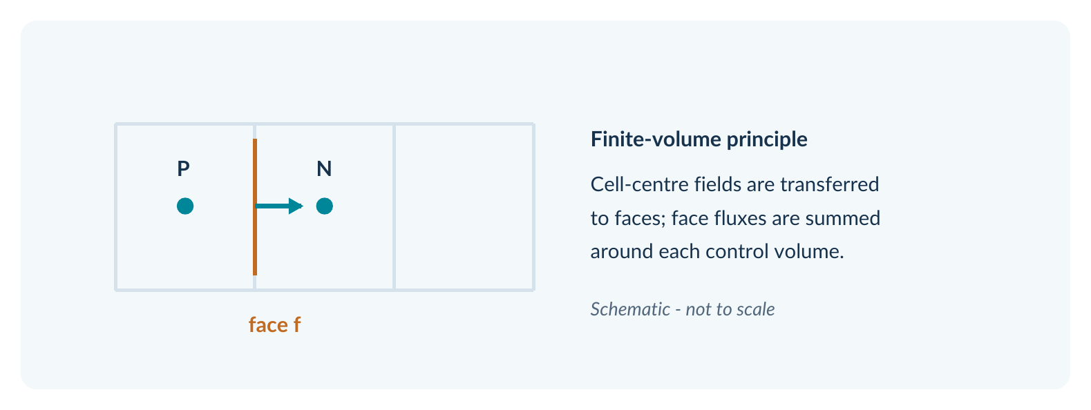
Interpret a common entry
Gauss integration + linear face interpolation:
gradSchemes
{
    default Gauss linear;
}
A Gauss gradient reconstructs the volume integral of a derivative through a surface sum. linear specifies how cell-centre values are interpolated to a face. These two words describe different stages of the operation.
A useful mental model
- Choose how a value is represented at the face.
- Evaluate a flux or a face contribution.
- Sum face contributions to form a cell equation.
- Assemble the resulting algebraic system for the solver.
Optional refresher · Cell-to-face values
For two adjacent cells P and N, a linear face value is a geometry-weighted interpolation between the two cell values. Equal weights apply only in a symmetric geometric situation.
Deep dive · The Gauss gradient in formulas and numbers
Gauss’s theorem applied to the gradient states that the integral of ∇a over a cell volume equals the integral of a·n over its surface. Approximating the mean gradient by its centre value and the surface integral by a sum over faces:
(∇a)_P ≈ (1 / V_P) Σ_f S_f a_f          S_f = face area vector (outward, magnitude = face area)
a_f = w a_P + (1 − w) a_N               linear interpolation, w = weight of the owner cell
In OpenFOAM the linear weight is computed from the distances of the two centres from the face plane, measured along the normal: w = dfN/(dPf + dfN). Example: centre P at x = 0, centre N at x = 3 mm, face at x = 1 mm (cell P smaller). Then dPf = 1 mm, dfN = 2 mm, w = 2/3: the face, closer to P, takes 2/3 of P’s value. With aP = 1 and aN = 4 we get af = (2/3)·1 + (1/3)·4 = 2, which is exactly the value of the linear function a(x) = 1 + x (in mm) at x = 1 mm. The scheme gets its name from this: it is exact for linear variations, hence second-order accurate.
On boundary faces there is no cell N: the face value is that of the patch boundary condition (Part 3). This is where the conditions in 0/U and 0/p enter the discrete operators: a fixedValue supplies af directly, a zeroGradient sets af = aP.
Deep dive · From face contribution to sparse matrix
Steps 3 and 4 of the mental model have a very concrete structure in OpenFOAM. The system matrix (class fvMatrix, based on lduMatrix) stores a diagonal (one value per cell) and two off-diagonal coefficient vectors, “upper” and “lower”, one per internal face. Each internal face links the owner cell to the neighbour and carries its coefficient into both rows. For example, for diffusion between P and N with face coefficient Γf|Sf|/|d|:
row P:   diag_P   −= Γ_f |S_f| / |d|      coefficient of N in row P = + Γ_f |S_f| / |d|
row N:   diag_N   −= Γ_f |S_f| / |d|      coefficient of P in row N = + Γ_f |S_f| / |d|
The number of off-diagonal coefficients is therefore twice the number of internal faces, and the sparsity pattern of the matrix is the mesh topology. For the channel of Part 2 (40 × 10 × 5 = 2000 cells, 5350 internal faces) the matrix has 2000 diagonal entries and 10700 off-diagonal ones, out of 4 million possible positions: 0.3 %. This sparsity is what makes the iterative solvers of Part 6 possible.
7. gradSchemes: gradients and limiting
Gradients are used in momentum and pressure operations, in stress evaluation, and sometimes in higher-order convection reconstruction. A frequently used v14 default is:
Common gradient setting:
gradSchemes
{
    default Gauss linear;
}
The name describes Gauss integration together with linear interpolation. An alternative seen in the Foundation v14 guide is leastSquares, which fits local variation using neighbouring cell information.
Why limit a gradient?
Extrapolating a reconstructed gradient from the centre to the face may overshoot neighbouring values. A limiter reduces the reconstructed gradient where that risk occurs, which can improve robustness at the cost of additional numerical diffusion.
Explicitly limit only the velocity gradient:
gradSchemes
{
    default Gauss linear;
    grad(U) cellLimited Gauss linear 1;
}| Configuration | Meaning |
|---|---|
default Gauss linear; | Use the standard gradient for unspecified terms. |
grad(U) ... | Override only the gradient of velocity. |
cellLimited ... 1 | Apply the documented strong cell-based limiting setting. |
Optional refresher · Gradient versus divergence
A scalar gradient is a vector; divergence of a vector is a scalar. The names identify different mathematical operations even when both use face integrals.
Deep dive · Gauss linear versus leastSquares
Gauss linear uses only the faces of the cell and the values interpolated on them; it is cheap, conservative in form and exact for linear fields on regular meshes. On strongly distorted meshes (strong asymmetry between cells, i.e. skewness, or cells with very different faces) linear interpolation does not happen at the face centre and accuracy degrades. leastSquares instead chooses the gradient that minimises, in a weighted least-squares sense, the difference between aN − aP and (∇a)P·dPN over all neighbouring cells: it is exact for linear fields on any mesh and therefore more robust with skewness, but tends to be more sensitive on highly stretched cells and costs more.
The v14 User Guide gives Gauss linear as the usual choice and mentions leastSquares and Gauss cubic as rarely used alternatives. For the regular hexahedral channel the two choices give the same gradient up to round-off in interior cells: a good sanity test, not an interesting experiment.
Deep dive · How cellLimited works and what the coefficient means
The cellLimited limiter first computes the gradient with the scheme that follows it (here Gauss linear), then checks each cell: for each face it extrapolates the value aP + (∇a)P·(xf − xP) and checks that it does not leave the [min, max] range of the values of the cell and its neighbours. If it does, it multiplies the whole cell gradient by the factor (≤ 1) that brings the worst extrapolation back inside the range. The final coefficient, between 0 and 1, sets how much margin is allowed: 1 enforces the bound strictly (the “strong limiting” of the table), 0 is equivalent to no limiting.
Example. In a row of cells with 1 mm spacing the values are 0, 1, 1 (W, P, E). The central gradient at P is (1 − 0)/2 = 0.5 per mm. Extrapolated to the east face (0.5 mm) it gives 1 + 0.25 = 1.25: it exceeds the local maximum 1. The limiter reduces the gradient to 0 in that cell (the only factor that does not exceed 1 on the east side), and the face value becomes 1. Without a limiter, a scheme such as linearUpwind that uses this gradient would create a new maximum, i.e. a non-physical oscillation.
The v14 User Guide shows cellLimited Gauss linear 1 for velocity and turbulence gradients (grad(U), grad(k), grad(epsilon)) to maintain boundedness on poor-quality meshes. The OpenFOAM source code also contains variants such as cellMDLimited (directional limiting, less diffusive) and faceLimited; they are not covered by the guide, so before using them check in your installation that they exist (for example with the “Valid schemes” list described in the opening section) and look for a tutorial that uses them.
Deep dive · Named gradients and the reference from linearUpwind
The argument of linearUpwind (section 8) is not a formula but the name of a gradSchemes entry: linearUpwind grad(U) means “for the reconstruction use the gradient defined by gradSchemes/grad(U), or by the default if missing”. It follows that an override such as grad(U) cellLimited Gauss linear 1; also acts on the convective reconstruction of velocity. Some Foundation tutorials exploit this mechanism by defining an entry with a free name in gradSchemes, for example limited cellLimited Gauss linear 1;, and recalling it in divSchemes as linearUpwind limited: velocity then uses a limited gradient only in the convective reconstruction, while other uses of grad(U) remain unlimited. Before copying this pattern, check with foamSearch how the tutorial of your version writes it.
8. divSchemes: what div(phi,U) means
In the incompressible constant-density context, phi typically represents the volumetric flux through each face. In a finite-volume momentum equation, div(phi,U) labels the transport of velocity by this face flux.
Representative v14 incompressibleFluid entries:
divSchemes
{
    default none;
    div(phi,U) Gauss linearUpwind grad(U);
    div((nuEff*dev2(T(grad(U))))) Gauss linear;
}| Entry | Physical/numerical role |
|---|---|
div(phi,U) | Convection of velocity by the face flux phi. |
Gauss | Conservative face-summation discretisation. |
linearUpwind | Upwind-biased higher-order face reconstruction. |
grad(U) | Gradient expression needed by that reconstruction. |
div((nuEff*...)) | Divergence of a viscous stress-related expression; not advection. |
Read div(phi,U) as one operator name. Do not assume that every div(...) entry uses the same flux interpolation or describes convection.
Optional refresher · Convective flux
A face mass or volumetric flux specifies how much material crosses a surface. The value of the transported field at that face then determines the transported momentum or scalar quantity.
Deep dive · What phi is, in units and numbers
phi is a surface field (surfaceScalarField): one number per face, Ff = Sf·Uf, with dimensions [m³/s] in incompressible modules. In compressible modules the same name denotes the mass flux ρSf·Uf [kg/s], which is why the same string div(phi,U) can have a slightly different physical meaning depending on the module. The module creates phi at start-up from the initial velocity (or reads it if a phi file exists in the start-time directory) and updates it after each pressure correction so that it satisfies discrete continuity; when results are written a phi file appears in every time directory.
Channel numbers. An inlet face of the Part 2 mesh measures 1 mm × 1 mm = 1.0 × 10⁻⁶ m²; at U = 0.05 m/s its flux is 5.0 × 10⁻⁸ m³/s, and the 50 inlet faces add up to 2.5 × 10⁻⁶ m³/s, the channel flow rate. The convective contribution of a face to the momentum equation is Ff·Uf: a momentum flux (per unit density) [m⁴/s²]. The scheme in div(phi,U) decides only Uf; Ff comes from the pressure–velocity coupling.
The flux can be inspected like any other field: foamDictionary -entry internalField 0.02/phi | head shows the first values (one per internal face, in face order), and the sum over patches can be computed with the patchFlowRate function object, which can be run afterwards, for example with foamPostProcess -func "patchFlowRate(patch=outlet)" -latestTime (check the exact arguments with foamPostProcess -list and with the file under $FOAM_ETC/caseDicts/functions).
Deep dive · Why the second divergence uses Gauss linear
In the entry div((nuEff*dev2(T(grad(U))))) the field whose divergence is computed is an already known tensor, evaluated explicitly from current values: νeff times the deviatoric part of the transposed velocity gradient. There is no “direction of transport” and no flux carrying information from upstream: it is a diffusive quantity, so second-order central linear interpolation is the natural choice. Upwind schemes would make no sense: upwind itself needs a flux to know which cell is upstream, and there is none here.
For the algebra: ∇·[ν(∇U + (∇U)T)] = ∇·(ν∇U) + ∇·[ν(∇U)T]. With constant ν and ∇·U = 0 the second term vanishes exactly (it equals ν∇(∇·U)), but in discrete form, with variable νeff (turbulence) or continuity not yet satisfied, it is not zero. The v14 User Guide states that non-advective terms in divSchemes typically use Gauss linear. Non-linear models add similar entries (for example a divergence of non-linear stresses): same reasoning, same scheme.
9. Comparing the common convection schemes
There is no generally optimal convection scheme. Higher formal order can reduce truncation error, whereas stronger limiting may suppress non-physical oscillations in demanding regions of the mesh.
| Scheme | Character | Risk / trade-off |
|---|---|---|
Gauss upwind | First-order, upwind cell selection. | Bounded and robust but numerically diffusive. |
Gauss linear | Second-order central interpolation. | Less numerical diffusion but unbounded. |
Gauss linearUpwind grad(U) | Higher-order upwind-biased reconstruction. | Requires gradient; can remain unbounded. |
Gauss limitedLinear 1 | Linearly interpolated solution with limiter. | More robust near sharp variation; can add diffusion. |
Gauss LUST grad(U) | 75% linear / 25% linearUpwind blend. | Still requires checking stability and accuracy. |
Mutually exclusive choices:
// Controlled A/B test, change only this one line:
div(phi,U) Gauss upwind;
// versus
div(phi,U) Gauss linearUpwind grad(U);
Interpretation: if two simulations differ, the change may come from both spatial truncation error and nonlinear response. A changed picture is not automatically a more physically accurate result.
Optional refresher · Numerical diffusion
First-order upwind can smear steep transported profiles. A less diffusive higher-order scheme can retain detail but may create oscillations unless the overall scheme/model/mesh controls them.
Deep dive · Five schemes on the same face: a numerical example
Uniform one-dimensional mesh, spacing Δx, positive flow (left to right). Three consecutive cells W, P, N with values aW = 0, aP = 1, aN = 3; we want the value on face f between P and N. Since the flow goes from P to N, the upwind cell is P.
| Scheme | Formula | af |
|---|---|---|
upwind | af = aP | 1 |
linear | af = (aP + aN)/2 | 2 |
linearUpwind | af = aP + (∇a)P·Δx/2, with (∇a)P = (aN − aW)/(2Δx) | 1 + 0.75 = 1.75 |
LUST | 0.75·linear + 0.25·linearUpwind | 1.5 + 0.4375 = 1.9375 |
limitedLinear 1 | between upwind and linear, according to a limiter function of the gradient ratio r | here r = 0.5: with the Sweby-type limiter, ψ = min(2r/k, 1) = 1 → 2 |
The ratio r compares the upwind slope (aP − aW = 1) with the slope across the face (aN − aP = 2). Where the profile is smooth (r close to 1 or, as here, not too small) limitedLinear behaves like linear; where the slope changes abruptly or reverses (r ≤ 0, i.e. a local maximum or minimum) it falls back to upwind, which cannot create new extrema. According to the v14 User Guide the coefficient 1 gives the strongest limiting; smaller values (towards 0) limit less. The exact limiter formula should be taken from the source code; the example is meant to show its behaviour, not to replace it.
The four different answers (1; 1.75; 1.94; 2) show why the choice matters: the face value multiplies the flux Ff and therefore changes the transported momentum. Godunov’s theorem explains why no perfect scheme exists: no linear scheme of higher than first order can be monotone (free of new oscillations). Limited schemes get around the theorem by being non-linear: their weighting depends on the solution itself.
Deep dive · How much numerical diffusion upwind adds in the channel
A Taylor-series expansion shows that the upwind scheme solves, instead of the original equation, an equation with an extra diffusion of about Γnum ≈ |U|Δx/2 in the flow direction. For the channel (U = 0.05 m/s, Δx = 2.5 mm) Γnum ≈ 6.3 × 10⁻⁵ m²/s, about 60 times the physical viscosity ν = 1.0 × 10⁻⁶ m²/s. The same comparison can be expressed with the cell Péclet number, Pe = UΔx/ν = 125: when Pe ≫ 2, upwind numerical diffusion dominates the physical one.
This does not mean the channel results will be wrong by a factor of 60. Numerical diffusion acts where the transported field varies along the flow direction; in the developed part of a channel the velocity profile hardly changes along x, and the convective term is small. Differences between upwind and linearUpwind are therefore expected mainly in the inlet region, where the uniform profile turns into the parabolic one, and in early transients. It is a prediction to be checked in the laboratory of section 15, not a guaranteed result.
Deep dive · Other v14 guide schemes: V variants, vanLeer, 01 and multivariate
- V variants (
limitedLinearV 1,linearUpwindV grad(U)): for vector fields, they use a single limiter for all components, computed in the direction of greatest change, instead of limiting each component separately. The v14 User Guide gives examples fordiv(phi,U), also with theboundedprefix. vanLeer,vanAlbada: other limited TVD-type schemes, used mainly for scalars.01variants (for examplelimitedLinear01 1): bound more strictly between 0 and 1, for scalars that by definition lie in that range (fractions, progress variables).multivariateSelection: applies one common limiter to several coupled equations, for example species mass fractions and enthalpy, so that they stay mutually consistent.
These are all tools for specific problems; for the laminar channel with velocity only, the five schemes in the table are more than enough. The appendix rule still holds: start from a native v14 tutorial with similar physics and record every deviation.
10. What the bounded prefix changes
Foundation v14 supports bounded variants of several Gauss convection schemes. The prefix does not mean “more physically accurate” and is not interchangeable with choosing a limiter such as limitedLinear.
Two contexts; do not combine the lines:
// Often seen in steady-state examples:
div(phi,U) bounded Gauss linearUpwind grad(U);
// An ordinary transient alternative:
div(phi,U) Gauss linearUpwind grad(U);
For incompressible flow, the advective derivative can be written as a conservative divergence plus a term involving div(U). At exact continuity, that correction vanishes; during iterative convergence, discrete continuity is not yet exact. The bounded formulation accounts for that discrepancy.
Three distinct concepts
| Term | What it controls |
|---|---|
bounded | Modification of the convective operator relevant to discrete continuity. |
limitedLinear | Limiter acting on the interpolated convected field. |
steadyState | Removal of time derivatives in ddtSchemes. |
Optional refresher · The algebra
For a scalar a: U · grad(a) = div(U a) − a div(U). The extra term is zero for an exactly divergence-free velocity; it can matter during convergence to an incompressible solution.
Practice: follow the bounded/unbounded choice in a native v14 tutorial suited to the same run regime before experimenting.
Deep dive · What bounded does in the discrete system
In discrete form, the div(U) term of a cell is the sum of outgoing fluxes divided by the volume: (Σf Ff)/VP. The bounded Gauss … operator first builds the convection with the given scheme and then implicitly subtracts aP·Σf Ff, i.e. the a·div(U) term of the identity: in practice it adds −ΣfFf to the cell diagonal. If continuity is exact, Σf Ff = 0 and nothing changes; if it is not, the term compensates for the cell’s mass imbalance.
Why it is needed. Imagine a cell into which, halfway through convergence, more flux enters than leaves: Σf Ff = −1 × 10⁻⁹ m³/s. In the purely conservative form the cell “accumulates” the transported quantity in proportion to the imbalance, as if there were a fictitious source; in steady iterations, where there is no V/Δt term to damp it, this spurious source can push a field outside its physical bounds (for example a negative turbulence quantity). By subtracting a·div(U) the operator becomes the non-conservative form U·∇a, which cannot create new extrema because of the continuity error. The v14 User Guide states that this helps maintain the boundedness of the solution variable and promotes better convergence, especially in steady-state runs.
In transient runs, with PIMPLE converged at each step, continuity is satisfied to within the pressure solver tolerance, the term is negligible and the conservative form is preferable: that is why the transient line of this section has no prefix. The prefix combines with any convection scheme (bounded Gauss upwind, bounded Gauss limitedLinear 1, bounded Gauss linearUpwindV grad(U)…) and does not replace the limiter: they are two independent corrections.
11. laplacianSchemes: diffusion
Diffusive terms involve gradients normal to faces. For Laplacian-type operators, Foundation v14 uses the Gauss construction with an interpolation scheme for the diffusion coefficient and a surface-normal gradient scheme.
Common teaching baseline:
laplacianSchemes
{
    default Gauss linear corrected;
}
Decode each word
| Word | Meaning |
|---|---|
Gauss | Assemble the diffusion operator using surface contributions. |
linear | Interpolate the diffusion coefficient to the faces. |
corrected | Correct the normal gradient for mesh non-orthogonality. |
The scheme applies to the Laplacian operators requested by the active equations. Separate entries may also be used for particular operators; the mathematical identifier must match the one the solver assembles.
Example from v14 guidance:
// Alternative correction policy, not a universal improvement:
default Gauss linear limited corrected 0.5;
Optional refresher · Diffusion
The form div(Gamma grad(a)) describes transport driven by gradients. The coefficient Gamma can vary spatially; face interpolation is then needed before evaluating the flux.
Deep dive · The discrete Laplacian formula and a channel example
Integrating ∇·(Γ∇a) over the cell and applying Gauss gives a sum of face diffusive fluxes: Σf Γf |Sf| (∂a/∂n)f. The three words of the entry correspond exactly to the three factors: Gauss is the sum, linear provides Γf, corrected provides (∂a/∂n)f. On an orthogonal mesh the normal gradient is simply (aN − aP)/|d|, with |d| the distance between centres, and the implicit part goes entirely into the matrix.
Example. Face between two channel cells stacked in y (Part 2 mesh: |Sf| = 2.5 mm × 1 mm = 2.5 × 10⁻⁶ m², |d| = 1 mm). With ν = 1.0 × 10⁻⁶ m²/s the face coefficient is ν|Sf|/|d| = 1.0 × 10−6 · 2.5 × 10−6/1.0 × 10−3 = 2.5 × 10⁻⁹ m³/s. If the axial velocities of the two cells are 0.060 and 0.066 m/s, the diffusive momentum flux across the face is 2.5 × 10−9 · 0.006 = 1.5 × 10⁻¹¹ m⁴/s²: this exchange, summed over all faces, is what produces the channel pressure drop.
According to the v14 User Guide, Gauss is the only choice available for Laplacians, in the form Gauss <interpolation scheme> <snGrad scheme>: that is why the entry always has three parts (four if the snGrad scheme takes a coefficient, as in limited corrected 0.5). The channel’s Laplacian operators are laplacian(nuEff,U) in the momentum equation and a pressure Laplacian whose name contains the coefficient built by the pressure–velocity algorithm; with a default there is no need to know it, but if default none is used the error message reports it exactly.
Deep dive · When linear is not enough for the coefficient
In the channel ν is uniform and the interpolation of the coefficient is irrelevant: any average of two equal values gives the same number. It becomes important when Γ varies strongly from cell to cell: turbulent viscosity near walls, thermal conductivity at the interface between two materials in a multi-region case, permeability in a porous medium. In a series conduction problem between two layers, the correct flux across the interface is governed by the harmonic mean of the conductivities, not the arithmetic one: with ΓP = 1 and ΓN = 100 the linear mean gives ≈ 50.5, the harmonic one 2/(1/1 + 1/100) ≈ 1.98, a 25-fold difference in the face flux. OpenFOAM has a harmonic interpolation scheme for such cases; before using it, check in a relevant v14 tutorial that it is used with that syntax.
12. snGradSchemes and mesh geometry
A surface-normal gradient is the derivative component perpendicular to a cell face. On a non-orthogonal mesh, the line joining neighbouring cell centres is not aligned with that normal.
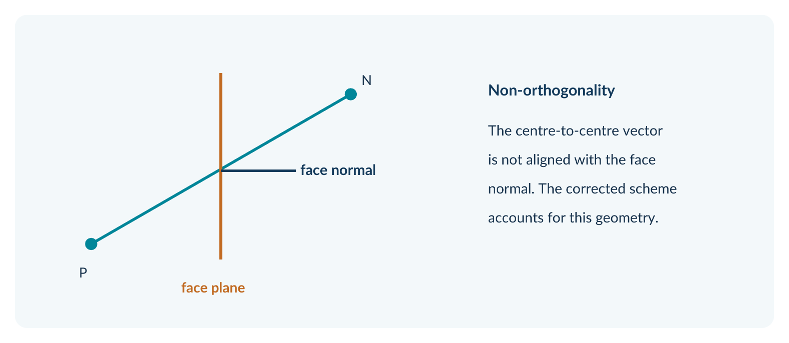
corrected scheme accounts for this geometry.Compare geometrically motivated options:
snGradSchemes { default corrected; }
// One optional limited-correction alternative:
snGradSchemes { default limited corrected 0.5; }
corrected adds the contribution associated with non-orthogonality. limited corrected constrains that contribution. The appropriate treatment must be considered together with checkMesh and the whole numerical model.
Design caution
For the one-block orthogonal channel, switching to a non-orthogonal correction policy may have little measurable impact. A skewed or strongly non-orthogonal mesh is not a safe place to make arbitrary stability experiments.
Deep dive · How OpenFOAM decomposes the normal gradient
Let d be the vector from P to N and Sf the face area vector. If d is parallel to Sf (orthogonal mesh), the normal gradient is exactly (aN − aP)/|d| to second order. If not, OpenFOAM splits Sf into two parts: one parallel to d, Δ, treated implicitly with the difference between the two centres, and a correction k = Sf − Δ, multiplied by the gradient interpolated to the face (∇a)f and treated explicitly:
S_f · (∇a)_f  ≈  |Δ| (a_N − a_P) / |d|   +   k · (∇a)_f
                  implicit (matrix)           explicit (non-orthogonal correction)

over-relaxed decomposition:  Δ = d (S_f · S_f) / (d · S_f)
The explicit part uses the gradient of the current solution, so it is exact only if it is recomputed after solving: that is the reason for the non-orthogonal correctors (nNonOrthogonalCorrectors in fvSolution, Part 6), which repeat the solution of the pressure equation while updating the correction. On an orthogonal mesh k = 0 and the correction does nothing: corrected and orthogonal give the same result, and extra correctors are just wasted computing time.
Deep dive · The four v14 guide options and the meaning of the limited coefficient
| Scheme | Behaviour according to the v14 User Guide |
|---|---|
orthogonal | Second-order only if the centre-to-centre vector is orthogonal to the face; no correction. |
uncorrected | The corrected scheme without the non-orthogonal correction; like orthogonal, suitable only for very low non-orthogonality (up to about 5°). |
corrected | Adds the explicit non-orthogonal correction; generally the recommended choice. |
limited corrected ψ | Limits the correction: 0.33 more stable, 0.5 more accurate. Limiting may be needed above about 75° non-orthogonality; above about 85° convergence becomes difficult. |
The coefficient ψ of limited (between 0 and 1) limits the explicit correction relative to the orthogonal part: the correction cannot exceed ψ/(1 − ψ) times the implicit part. With ψ = 0.5 the correction can at most equal the orthogonal part; with ψ = 0.33 it can be at most about half of it; ψ = 0 is equivalent to uncorrected and ψ = 1 to corrected. Limiting trades some accuracy on highly distorted cells for the stability of the explicit correction, which on faces almost tangent to the vector d can become dominant.
Deep dive · Reading non-orthogonality with checkMesh before choosing
checkMesh reports the non-orthogonality angle, i.e. the angle between d and Sf, in the form Mesh non-orthogonality Max: … average: …, and flags as errors the faces beyond its default threshold of 70°. For the single-block straight blockMesh channel the expected result is Max: 0 average: 0: all faces are perfectly orthogonal. For an unstructured mesh generated with Gmsh (the Gmsh and gmshToFoam channel case) the values are typically non-zero and must be read before choosing snGradSchemes and the number of non-orthogonal correctors.
checkMesh > log.checkMesh 2>&1
grep -i "non-orthogonality" log.checkMesh
grep -i "skewness" log.checkMesh- Max < about 5°:
correctedandorthogonal/uncorrectedare practically equivalent;correctedremains the safest choice. - Max up to about 70°:
corrected, possibly with one or two non-orthogonal correctors. - Max above about 75°: consider
limited corrected 0.5or0.33(and the same policy inlaplacianSchemes), but first ask whether the mesh should be improved. - Max above about 85°: convergence becomes difficult; the remedy lies in the mesh, not in the schemes.
The thresholds are those given by the v14 User Guide and by checkMesh; they are guidelines, not hard rules. The correction policy in snGradSchemes and the one in the last word of laplacianSchemes should be consistent with each other.
13. interpolationSchemes and wallDist
Two additional sections commonly appear in v14 examples even though they do not correspond to a named term in the simplest PDE diagram.
Interpolation between cell centres and faces
General face interpolation:
interpolationSchemes
{
    default linear;
}
This sets the default for interpolation operations not already specified by a more specialised discretisation entry. The Foundation v14 guide notes that linear is used in almost all supplied tutorial cases.
Distance to the nearest wall
Optional when a model requests wall-distance data:
wallDist
{
    method meshWave;
}
wallDist is a configuration for the method of evaluating distance to walls, relevant to models that require that quantity. It is not a universal mandatory part of every laminar fvSchemes file.
What is not in this part?
d2dt2Schemesapplies when second temporal derivatives are used; it is not needed for the channel baseline.- Transport of species, energy and turbulence quantities introduces further field-specific divergence names.
- Specialised higher-order and multivariate limiters can be studied after mastering the main operator families.
Note for the reactor project
Wall-distance and convection settings from a RANS tutorial cannot be transferred blindly to a laminar expanded-mesh reactor simulation. The governing equations and active models determine which entries matter.
Deep dive · Where interpolationSchemes is used in the channel
The interpolations “already specified by a more specialised entry” are those inside other schemes: the linear of Gauss linear in gradSchemes, the convection scheme in divSchemes, the coefficient interpolation in laplacianSchemes. What remains are the “bare” interpolations the module requests explicitly, the most important of which in incompressibleFluid is building the face flux from the predicted velocity in the pressure-correction step. The initial computation of phi from the initial velocity also uses a cell-to-face interpolation.
Changing this default in an incompressibleFluid case therefore modifies the pressure–velocity coupling, not convection: an experiment best avoided without a precise reason. The v14 User Guide mentions the use of cubic in one stress-analysis tutorial as an exception.
Deep dive · wallDist: who asks for it and what happens if it is missing
The wall distance y is a volume field used directly by some turbulence models: Spalart–Allmaras (the airFoil2D model), k-ω SST (in its blending functions), LES models with wall damping. In the laminar channel no model needs it, so the sub-dictionary can be missing without consequences. If a model does need it and wallDist is missing, the run stops at start-up with an error reporting the missing entry in system/fvSchemes: the fix is to add it, not to change model.
meshWave computes the distance by propagating information from the wall faces through the mesh, cell by cell: it is fast and robust, and it is the tutorial method. Other run-time selectable methods exist, for example based on solving a Poisson equation, which are smoother on highly distorted meshes; the authentic list for your installation is obtained from the “unknown method” error or with foamToC -search meshWave.
Deep dive · d2dt2Schemes and divergence names in richer cases
The second time derivative, ∂²a/∂t², appears in solid dynamics equations (for example the displacement in the stress-analysis module). According to the v14 User Guide, only Euler is available for d2dt2Schemes. It is never needed for fluids.
Each additional transport equation brings at least one divergence with its own name: a k-ε model adds div(phi,k) and div(phi,epsilon), a k-ω model div(phi,omega), the energy equation a divergence of the energy variable chosen by the module, each species a divergence of its mass fraction. In compressible modules phi becomes a mass flux and terms such as the divergence of kinetic energy or of pressure work can appear. The reliable way to know the exact names is to read a native tutorial of the same module, or to let default none make them appear one at a time in the errors.
14. Guided laboratory: decode a real v14 file
Before editing the channel, inspect a native OpenFOAM 14 tutorial to see a dictionary written for a real solver module. One reference used for this part is incompressibleFluid/cylinder. Its fvSchemes contains additional model-dependent entries.
Step-by-step reading method
- Confirm the installed environment with
foamVersionand locate the tutorial directory. - Open
system/fvSchemesin a v14incompressibleFluidtutorial. - For each section, identify its
defaultand all explicit overrides. - Mark which entries are advection, which are stress divergence and which are auxiliary model settings.
- Look up at least one unfamiliar scheme in the v14 User Guide, Section 4.5.
- Write a short note explaining why
divSchemes/default nonedoes not mean “no advection is calculated”.
Read-only inspection commands · line continuation shown:
foamVersion
echo "$FOAM_TUTORIALS"
foamSearch "$FOAM_TUTORIALS" fvSchemes ddtSchemes/default
foamSearch "$FOAM_TUTORIALS" fvSchemes \
  "divSchemes/div(phi,U)"
The command output lists values found in tutorials; it is evidence of usage, not a recommendation for your present case.
Answer these before proceeding
- What is the difference between
div(phi,U)and the viscous stress-divergence entry? - Why does
linearUpwindinclude a gradient expression? - Which dictionary decides whether the case is transient? Which entry discretises its time derivative?
Deep dive · What to expect from the inspection commands
foamVersion must print version 14 (for example OpenFOAM-14): if it prints something else, or the command does not exist, the environment is not active and the following commands will use another installation or fail. echo "$FOAM_TUTORIALS" prints the path of the active installation’s tutorial directory; if the line is empty, the variable is undefined and the environment has not been loaded. foamSearch walks all fvSchemes files under that path, extracts the value of the requested entry and prints the sorted list of distinct values, one per line, in the form default Euler;, default steadyState; and so on. The exact length and content of the list depend on the installation: there is no “right” output to compare, there is an inventory to read.
To turn the inventory into information, trace the cases that use a given value and compare their regime. For example, to know which tutorials use bounded in the velocity convection and whether they are steady:
foamSearch -count "$FOAM_TUTORIALS" fvSchemes "divSchemes/div(phi,U)"
grep -l "bounded Gauss linearUpwind" "$FOAM_TUTORIALS"/incompressibleFluid/*/system/fvSchemes
for f in "$FOAM_TUTORIALS"/incompressibleFluid/*/system/fvSchemes; do
  printf "%s : %s\n" "$f" "$(foamDictionary -entry ddtSchemes/default -value "$f")"
done
You should expect to see bounded mainly in cases with steadyState: the rule of section 10 observed in the data rather than memorised.
Deep dive · The fvSchemes of incompressibleFluid/cylinder, entry by entry
In the version published in the OpenFOAM-14 repository (link in the appendix) the cylinder file contains, at the time of writing: ddtSchemes/default steadyState, with a comment pointing to Euler for transient use; gradSchemes with default Gauss linear and a cellLimited version for the velocity and turbulence gradients (U, k, omega, epsilon); divSchemes with default none, bounded velocity convection based on linearUpwind with a limited gradient, bounded convection with limitedLinear for the turbulence quantities (reused through a macro) and further entries intended for compressible modules, such as energy and pressure divergences; laplacianSchemes Gauss linear corrected, interpolationSchemes linear, snGradSchemes corrected and wallDist with meshWave. Open the installed file to check the exact syntax.
| Entry class (step 04) | Cylinder entries |
|---|---|
| Advection | div(phi,U) and the div(phi,…) divergences of the turbulence quantities and, in compressible modules, of energy. |
| Stress divergence | div((nuEff*dev2(T(grad(U))))) and its compressible variants. |
| Auxiliary model settings | wallDist, the macro entry for the turbulence scheme, the named gradient used by linearUpwind. |
The fact that a file contains entries for modules you are not using is not an error: entries that are never requested are ignored (section 1). It is a developer choice to make the file reusable.
Deep dive · Model answers to the three questions and to the step-06 note
div(phi,U)versus stress divergence. The first is the convective transport of momentum by the face fluxphi: it needs a scheme that knows which side the flow comes from (upwind, linearUpwind…). The second is the explicit part of the viscous stress divergence, ∇·[νeff dev2((∇U)T)]: there is no transport, the tensor is known, and the natural scheme isGauss linear.- Why
linearUpwindhas a gradient. It reconstructs the face value by extrapolating from the upwind cell centre: af = aP + (∇a)P·(xf − xP). The gradient serves this extrapolation, and the argument says whichgradSchemesentry to use to compute it. - Transient or steady. The nature of the problem is read in
fvSchemes:ddtSchemes/default(or a specificddt(U)entry) decides whether the time derivative exists (Euler,backward…) or is removed (steadyState).controlDictsetsdeltaTandendTime, but withsteadyStatethese count iterations, not seconds;fvSolutionselects the consistent algorithm (PIMPLE or SIMPLE). The complete answer is therefore: theddtSchemesentry offvSchemes, backed by consistent settings in the other two dictionaries. - Step-06 note.
default noneonly removes the fallback: it says “do not pick a scheme for a divergence I have not named”. Velocity advection is very much calculated, with the scheme explicitly assigned todiv(phi,U); if that entry were missing, the run would not start at all rather than continue without advection.
15. Guided laboratory: make an A/B comparison
Keep the channel from Part 4 and perform a strictly controlled comparison. Use two new case copies, so neither the original case nor a previous result history is overwritten.
Example workflow after substituting your actual case name:
cp -a channelCase channel_upwind
cp -a channelCase channel_linearUpwind
cd channel_upwind
foamDictionary -entry "divSchemes/div(phi,U)" \
  -value system/fvSchemes
Modify only the velocity-advection entry in the two copies. Ensure both cases have the same mesh, boundary conditions, physical model, timestep and other schemes.
| Copy A | Copy B |
|---|---|
Gauss upwind | Gauss linearUpwind grad(U) |
| First-order, more diffusive baseline. | Higher-order, gradient-dependent comparison. |
What to record
- Exact changed line and the full file/checksum if practical.
- Run status: completed or failed, and the first meaningful error if present.
- Velocity profiles at the same coordinates and physical times.
- A pressure-drop measure on exactly the same inlet/outlet sections.
- The mesh, time step, initial state, model and residual criteria used in both runs.
Important
This is a comparison of numerical choices, not proof that one result is experimentally correct. A mesh-refinement/time-step study or an analytical/experimental reference is needed before claiming improved accuracy.
Deep dive · The complete workflow, from copy to comparison
The block in this section shows the start of the workflow: two copies and reading the current entry. Here is a complete, verifiable version. foamDictionary -set changes the entry in the file without opening an editor and without touching the rest; diff proves that the two copies differ only in that line; the checksum fixes the exact state of the files in the experiment record.
# 0. Start from a clean, complete channel case (mesh, 0/, constant/, system/)
cd /path/to/your/run
cp -a channelCase channel_upwind
cp -a channelCase channel_linearUpwind

# 1. Change exactly one entry in each copy
foamDictionary -entry "divSchemes/div(phi,U)" -set "Gauss upwind" \
  channel_upwind/system/fvSchemes
foamDictionary -entry "divSchemes/div(phi,U)" -set "Gauss linearUpwind grad(U)" \
  channel_linearUpwind/system/fvSchemes

# 2. Prove that only that line differs
diff channel_upwind/system/fvSchemes channel_linearUpwind/system/fvSchemes
diff -r -q channel_upwind/constant channel_linearUpwind/constant
diff -r -q channel_upwind/0 channel_linearUpwind/0
sha256sum channel_*/system/fvSchemes > fvSchemes.sha256

# 3. Run each case in its own directory, keeping its log
(cd channel_upwind && foamRun > log.foamRun 2>&1)
(cd channel_linearUpwind && foamRun > log.foamRun 2>&1)
tail -n 5 channel_*/log.foamRun
Expected result. The diff output on the two fvSchemes must show a single changed line, the one for div(phi,U) (foamDictionary -set may reformat spacing and comments: that is why the comparison is between the two modified copies, which were treated the same way). The two diff -r -q on constant and 0 must print nothing. The last lines of the two logs must contain End, showing that the run reached endTime.
Beware of restarts. If channelCase already contains time directories and controlDict uses startFrom latestTime (Part 4), the copies restart from the last result of the original case, computed with the original scheme: the comparison would be biased. Before running, check with ls that each copy contains only 0/, or explicitly set startFrom startTime in both (the same change in both, recorded in the log book).
Deep dive · Extracting profiles and pressure drop the same way for both cases
Items 03 and 04 of the record require measurements made with the same tool, at the same positions and at the same times. In OpenFOAM 14 the natural tool is function objects run afterwards with foamPostProcess: graphUniform samples fields along a segment with equally spaced points, and patchAverage averages a field over a patch. With the reference p = 0 at the outlet (Part 3), the average of p over the inlet is directly the kinematic pressure drop.
# Same line, same time, both cases (adapt the coordinates to your mesh, in metres)
for c in channel_upwind channel_linearUpwind; do
  (cd "$c" && foamPostProcess -time 0.02 \
     -func "graphUniform(start=(0.08 0 0.0025), end=(0.08 0.01 0.0025), nPoints=50, fields=(U))")
  (cd "$c" && foamPostProcess -time 0.02 -func "patchAverage(name=inlet, fields=(p))")
done
The example coordinates assume the 100 × 10 × 5 mm channel with its origin at a corner, expressed in metres: a vertical segment at x = 80 mm, at mid-width. Check the real extent with checkMesh (line Overall domain bounding box) and the function-object arguments with foamPostProcess -list and the files under $FOAM_ETC/caseDicts/functions. Results are written to postProcessing/ inside each case, with the same file name: compare them with a plot or with paste.
Deep dive · What to expect, and at which time to compare
With the settings from Part 4 (Δt = 0.002 s, endTime 0.02 s) the run covers only the first 20 ms after an impulsive start. In that time the boundary layer grows by about √(νt) = √(1.0 × 10−6 · 0.02) ≈ 0.14 mm: the profile is still almost uniform, with thin layers near the walls. The viscous development time over the smaller half-width (2.5 mm) is of order (2.5 × 10⁻³)²/ν ≈ 6 s, and the channel through-flow time L/U = 2 s. A comparison at t = 0.02 s therefore mainly measures the start-up response; to compare the developed flow you need times of a few seconds (thousands of steps, still cheap on 2000 cells) or the steady version of exercise C.
Qualitatively, differences between upwind and linearUpwind are expected to concentrate where the field varies along the flow, i.e. in the inlet region, and to be small in the developed part (section 9). The Poiseuille reference from the first worked case and the mesh-convergence study are the tools to decide which of the two results is closer to the exact solution: the A/B comparison alone only says how much the numerical choice matters in this case.
16. When the solver reports an unknown scheme
A malformed or missing scheme must be diagnosed by following the specific operator reported, rather than changing all discretisation entries. The failed run is evidence about which term the module actually requested.
| Observed symptom | First checks |
|---|---|
Missing discretisation for a div(...) operator | Match the complete operator keyword in divSchemes; check default none. |
| Unknown scheme name | Check spelling and exact syntax in Foundation v14 sources/tutorials. |
| Scheme needs a gradient | Check the syntax required by linearUpwind/LUST and relevant gradSchemes entries. |
| Unstable or oscillatory field | Check mesh quality, BCs, time step, flux balance and scheme boundedness before switching choices. |
| Unchanged results after editing | Check that you edited the active case and compared matching times and locations. |
Recommended diagnostic loop
- Save the exact failing log.
- Find the first relevant FATAL ERROR or scheme-selection message.
- Locate the named operator in
system/fvSchemes. - Inspect a working native v14 tutorial for that operator.
- Change the smallest number of entries required, then rerun.
Inspect parsed entries before launching a costly run:
foamDictionary -entry "ddtSchemes/default" \
  -value system/fvSchemes
foamDictionary -entry "divSchemes/div(phi,U)" \
  -value system/fvSchemes
Do not destroy evidence
Do not delete the original case or overwrite past results to “fix” a numerical problem. Preserve logs and full dictionaries; use new case copies for experiments.
Deep dive · What the messages look like, symptom by symptom
OpenFOAM messages have a stable structure: a --> FOAM FATAL ERROR or --> FOAM FATAL IO ERROR line (the latter when the problem lies in reading a file), the error text, then the file and lines involved and the code function that raised it. The typical forms, with paths and line numbers that vary from case to case:
| Symptom | Typical message form | Reading |
|---|---|---|
| Missing entry | keyword div(phi,U) is undefined in dictionary ".../system/fvSchemes/divSchemes" | The key is the one to add, character for character. |
| Unknown name | Unknown discretisation scheme linearUpwnd + Valid schemes are : … | The list that follows is the authentic set of names accepted for that operator type. |
| Missing argument | read error at the end of the entry (for example an attempt to read past the end of the input); the exact text depends on the version | Typical of Gauss linearUpwind; without the gradient name or limitedLinear without coefficient. |
| Missing sub-dictionary | wallDist or gradSchemes entry undefined in system/fvSchemes | A model or operator needs a whole missing family. |
# first fatal message, with context
grep -n -m 1 -A 15 "FOAM FATAL" log.foamRun

# which scheme keyword was missing or unknown
grep -n -i -E "undefined|Unknown discretisation scheme|Valid schemes" log.foamRun

# what the file really contains, after macros and #include
foamDictionary -expand system/fvSchemes
Always read the first error: later ones are often consequences. And remember that the reported key is evidence of what the module requests; if it does not match what you expected (for example a turbulence term appears in a case you thought was laminar), the problem is not in fvSchemes but in the model selected in constant/.
Deep dive · Instability and unchanged results: the checks before touching the schemes
Unstable field. The order of checks in the table is deliberate: most divergences originate in the mesh, boundary conditions or time step, not in the scheme. In practice: checkMesh (non-orthogonality, skewness, aspect ratio); the conditions in 0/U and 0/p (Part 3), especially backflow at the outlet; the Courant number in the log (Courant Number mean: … max: …), which in a transient PIMPLE case should stay of order one or less; the flux balance (inflow equal to outflow); and only then the boundedness of the schemes, for example moving from linear to linearUpwind or adding cellLimited to the gradient. Noting the first step where a residual or the Courant number blows up often points to the region and the cause.
Unchanged results. The typical causes are trivial and frequent: you edited the fvSchemes of another copy (check pwd and the path in the command); the run restarted from an already computed time (startFrom latestTime); you are comparing the 0 directory or a different time; the modified entry is never requested (for example you changed div(phi,k) in a laminar case); or the change is real but its effect is small in that case, as in the developed part of the channel. The checksum and the file timestamps (ls -l --time-style=full-iso system/fvSchemes log.foamRun) tell you whether the log postdates the change.
17. Independent exercises
Complete these tasks before consulting the answer key. For each exercise, state your prediction before asking OpenFOAM to verify it.
Exercise A — Classify
Identify the appropriate sub-dictionary for each operation: (1) transient time derivative, (2) cell-face interpolation, (3) convection of U, (4) diffusion of a scalar, (5) gradient of pressure, (6) derivative normal to a face.
Exercise B — Read and predict
Exercise dictionary:
gradSchemes
{
    default Gauss linear;
    grad(U) cellLimited Gauss linear 1;
}
divSchemes
{
    default none;
    div(phi,U) Gauss upwind;
}
Which scheme applies to grad(p)? To grad(U)? What happens if an equation requests an additional, unspecified divergence?
Exercise C — Controlled conversion
Starting with the teaching transient fvSchemes from section 3, construct a candidate steady-state scheme configuration. Identify at least two considerations beyond simply replacing Euler with steadyState. Do not run until the solver controls in Part 6 have been checked.
Exercise D — Documentation search
Find two authentic Foundation v14 tutorial entries for div(phi,U) and explain their differences without using a generic internet example from a different OpenFOAM branch.
Deep dive · How to verify your predictions with OpenFOAM
“Asking OpenFOAM to verify” has an operational meaning for each exercise. For A, in a copy of the case: set default none in one family at a time and observe which key appears in the start-up error: that is evidence of which sub-dictionary serves each operator (restore immediately afterwards). For B: in the channel case, with that dictionary, the second divergence div((nuEff*dev2(T(grad(U))))) is not specified, so the correct prediction is a fatal missing-entry error; run and compare. For C: foamDictionary -entry ddtSchemes/default -value system/fvSchemes must return steadyState, and the log of a steady run shows “time” advancing by 1 at each iteration. For D: the search commands are in the solutions box.
18. Worked answers and reasoning
A — Classification
| Operation | Sub-dictionary |
|---|---|
| Time derivative | ddtSchemes |
| Cell-to-face interpolation | interpolationSchemes |
| Convection of U | divSchemes |
| Diffusion Laplacian | laplacianSchemes |
| Gradient of p | gradSchemes |
| Face-normal gradient | snGradSchemes |
B — Effective settings
grad(p) uses Gauss linear through the default. grad(U) uses the cell-limited override. div(phi,U) uses Gauss upwind. An additional divergence has no generic fallback because default none is specified; its required operator must be configured.
C — Conversion requires more than a time-scheme edit
- A steady equation uses
ddtSchemes/default steadyState; a transient equation uses an appropriate physical-time scheme. - The advection entry may use a
boundedform in steady-state practice, according to the v14 guide and native tutorials. - The pressure–velocity correction configuration in
fvSolutionmust be appropriate for the new regime. controlDictstill controls iterations/time directories, but the interpretation of “time” changes in a steady solution.
D — Finding trustworthy examples
A valid answer cites the exact native v14 tutorial, its directory and the matching div(phi,U) entry. Explain why the cases differ; do not rank their numerical choices out of context.
Deep dive · Exercise C worked out: a candidate steady fvSchemes
A candidate configuration consistent with the v14 guide and the airFoil2D tutorial changes two lines relative to the section-3 file: the time scheme and the bounded prefix on convection. Everything else stays identical, because the other families do not depend on the time regime.
ddtSchemes
{
    default     steadyState;
}
gradSchemes
{
    default     Gauss linear;
}
divSchemes
{
    default     none;
    div(phi,U)  bounded Gauss linearUpwind grad(U);
    div((nuEff*dev2(T(grad(U))))) Gauss linear;
}
laplacianSchemes
{
    default     Gauss linear corrected;
}
interpolationSchemes
{
    default     linear;
}
snGradSchemes
{
    default     corrected;
}fvSolution: you need the steady algorithm dictionary (SIMPLE, withresidualControlas the stopping criterion) and under-relaxation factors inrelaxationFactors, because the V/Δt term that stabilised the transient is gone (Part 6).controlDict:deltaT 1;,endTimeequal to the maximum number of iterations (for example 2000) andwriteIntervalexpressed in iterations; the module remainsincompressibleFluid(Part 4).- Convergence criterion: initial residuals below the chosen threshold and quantities of interest (pressure drop, downstream profile) no longer changing between iterations; falling residuals alone are not enough.
- Comparison with the transient: the steady solution must be compared with the developed transient (a few physical seconds, section 15), not with the state at 0.02 s.
Deep dive · Exercise D worked out: how to build the answer
The first step is the inventory, the second is tracing back to the files and their regime:
foamSearch "$FOAM_TUTORIALS" fvSchemes "divSchemes/div(phi,U)"
grep -l "div(phi,U)" "$FOAM_TUTORIALS"/incompressibleFluid/*/system/fvSchemes
foamDictionary -entry "divSchemes/div(phi,U)" -value \
  "$FOAM_TUTORIALS"/incompressibleFluid/airFoil2D/system/fvSchemes
foamDictionary -entry "ddtSchemes/default" -value \
  "$FOAM_TUTORIALS"/incompressibleFluid/airFoil2D/system/fvSchemes
An example verified in the OpenFOAM-14 repository: in incompressibleFluid/airFoil2D/system/fvSchemes the entry is div(phi,U) bounded Gauss linearUpwind grad(U); with ddtSchemes/default steadyState. The case is steady and turbulent (Spalart–Allmaras): the bounded prefix follows the rule of section 10, and the second-order linearUpwind scheme is a common choice for momentum. The second example should be chosen among the tutorials that foamSearch lists in your installation, ideally a transient one (ddtSchemes/default equal to Euler or backward): its div(phi,U) entry is expected to lack bounded, and the scheme to reflect the needs of the case (for example a low-diffusion scheme such as LUST in a run that resolves turbulent structures in time). The correct answer documents file, entry and regime for both and links the differences to the equations and regime, without declaring one of them “better”.
19. Final self-assessment and checklist
Use this checklist before beginning Part 6 (fvSolution). The unit is complete when these questions can be answered without blindly copying an unrelated tutorial.
- I can point to
system/fvSchemesand explain its role separately fromfvSolution. - I can identify which mathematical operators are configured by the six common scheme sub-dictionaries.
- I know the difference between a dictionary
defaultand an explicit override. - I can explain why
divSchemes/default noneis useful. - I understand the main properties of
upwind,linear,linearUpwindandlimitedLinear. - I can explain what
boundedmeans in the v14 convection formulation. - I know why
correctedappears in Laplacian and surface-normal schemes. - I can use
foamSearchto locate documented syntax in native tutorials. - I can compare two cases while preserving the original and varying only one setting.
The essential map
Know which layer answers which question:
PDE operator      ->  fvSchemes discretisation
Discrete matrix   ->  fvSolution linear solver
Run schedule      ->  controlDict
Physical fields   ->  0/ and constant/
Next unit · Part 6 — fvSolution
After choosing the discrete approximation, OpenFOAM must solve the resulting coupled systems. Part 6 explains fvSolution, residual tolerances, linear solver choices and PIMPLE/SIMPLE controls.
Deep dive · A summary sheet of the schemes covered
| Family | Teaching value | Alternatives covered | What it decides |
|---|---|---|---|
ddtSchemes | Euler | steadyState, backward, CrankNicolson 0.9, localEuler | Time order; transient or steady |
gradSchemes | Gauss linear | leastSquares, cellLimited Gauss linear 1 | Gradient accuracy and boundedness |
divSchemes | none + Gauss linearUpwind grad(U) | upwind, linear, limitedLinear 1, LUST grad(U), bounded, varianti V | Convected face value |
laplacianSchemes | Gauss linear corrected | Gauss linear limited corrected 0.5 | Face coefficient and normal gradient in diffusion |
interpolationSchemes | linear | (rarely anything else) | Generic cell-to-face interpolations |
snGradSchemes | corrected | orthogonal, uncorrected, limited corrected 0.33/0.5 | Non-orthogonal correction |
wallDist | meshWave | other selectable methods | Wall distance for models that need it |
Appendix · Official sources and navigation
This part uses the OpenFOAM Foundation / CFD Direct v14 naming and examples. Different OpenFOAM branches and older versions can differ in their solver modules and configuration conventions.
Primary source
OpenFOAM v14 User Guide, §4.5 — Numerical schemes
https://doc.cfd.direct/openfoam/user-guide-v14/fvschemes
Sections: 4.5.1 time schemes; 4.5.2 gradients; 4.5.3 divergences; 4.5.4 surface-normal gradients; 4.5.5 Laplacians; 4.5.6 interpolation.
Related v14 user-guide chapters
- §4.1 Case file structure
https://doc.cfd.direct/openfoam/user-guide-v14/case-file-structure - §4.4 Time and data I/O control
https://doc.cfd.direct/openfoam/user-guide-v14/controldict - §4.6 Solution and algorithm control
https://doc.cfd.direct/openfoam/user-guide-v14/fvsolution
Version-specific example files (OpenFOAM Foundation v14)
- incompressibleFluid / cylinder / fvSchemes
https://github.com/OpenFOAM/OpenFOAM-14/blob/master/tutorials/incompressibleFluid/cylinder/system/fvSchemes - incompressibleFluid / airFoil2D / fvSchemes
https://github.com/OpenFOAM/OpenFOAM-14/blob/master/tutorials/incompressibleFluid/airFoil2D/system/fvSchemes
How to read the documentation efficiently
- Begin from a mathematical operator or field name, not a vaguely remembered scheme keyword.
- Look up the corresponding §4.5 subsection and its exact syntax.
- Search the installed
$FOAM_TUTORIALSfor a relevant v14 example. - Check that its flow regime, model and boundary conditions match the current problem.
- Record the reason for any deviation and test it on a copy of the case.
Deep dive · Reading the sources when the guide is not enough
The User Guide describes the most used schemes; the complete list and the exact behaviour are in the code. In a v14 installation the finite-volume schemes live under $FOAM_SRC/finiteVolume/interpolation/surfaceInterpolation/schemes (interpolation and convection schemes, for example linearUpwind, LUST, limitedLinear), $FOAM_SRC/finiteVolume/finiteVolume/gradSchemes (gradients and limiters), $FOAM_SRC/finiteVolume/finiteVolume/snGradSchemes, $FOAM_SRC/finiteVolume/finiteVolume/ddtSchemes, $FOAM_SRC/finiteVolume/finiteVolume/convectionSchemes (where the bounded variant also lives) and $FOAM_SRC/finiteVolume/finiteVolume/laplacianSchemes. The header of each .H file contains a description and, often, the usage syntax. A quick way to get oriented:
ls "$FOAM_SRC"/finiteVolume/finiteVolume/ddtSchemes
find "$FOAM_SRC"/finiteVolume -name "linearUpwind*.H"
sed -n '1,80p' "$(find "$FOAM_SRC"/finiteVolume -name linearUpwind.H | head -1)"
If your installation’s directory layout differs, find "$FOAM_SRC" -name "<name>.H" still finds the file. It is the same principle as the whole part: the evidence lies in the v14 installation you will use, not in a source from another branch.
Next part: OpenFOAM 14 Part 6: fvSolution, Linear Solvers and Solution Algorithms. Previous part: OpenFOAM 14 Part 4: controlDict and Simulation Control. Back to the Learning OpenFOAM 14 project index.