

OpenFOAM 14 Part 3: Fields, Initial Conditions and Boundary Conditions
Part 3 of 8 of the case-building series in Learning OpenFOAM 14. Part 2 used blockMesh to build the rectangular trainingChannel and its patches inlet, outlet and walls; this part gives those patches a physical meaning by writing the fields 0/U and 0/p.
From mesh patches to physical meaning. The subject is how to write and reason about the fields 0/U and 0/p in OpenFOAM Foundation 14, how to connect them to mesh patches, how to diagnose configuration errors and how to verify the result. Each “Deep dive” box expands a point with the theory, the v14 implementation, the alternatives and the practical checks.
How to use this part
Prerequisites. This part assumes the initial seven-step CFD workflow, applied in the first worked case (laminar channel flow and Poiseuille validation), and the preceding units on case structure (Part 1) and mesh (Part 2).
Scope. OpenFOAM Foundation 14. How to write and reason about the fields 0/U and 0/p, connect them to mesh patches, diagnose configuration errors, and verify the result.
Path through this part
Main track: physics → files → patch mapping → full 0/U and 0/p → checks → exercises. The Optional refresher boxes contain background material and can be skipped by readers already fluent in CFD.
Reference case: 3D laminar rectangular channel | Source guide: doc.cfd.direct/openfoam/user-guide-v14.
Learning contract
This unit does not introduce a new solver. It teaches the configuration layer that gives mathematical meaning to an already meshed CFD domain. At the end, you should be able to write the two field files without copying a whole tutorial.
What you should already have
- A working OpenFOAM 14 shell environment;
foamVersionshould identify version 14. - The channel mesh from Part 2, preferably a simple single-block mesh.
- Basic familiarity with dictionary syntax and with
blockMeshandcheckMesh. - A separate editable copy of the training case, never the original/reference case.
Outcomes and boundaries
By the end, you will distinguish internalField from boundaryField, identify the field class and dimensions, assign U and p conditions to all patches, and trace an input error back to its source.
Not in this unit
Mesh generation is covered in Part 2; time control, finite-volume schemes and algebraic solvers belong to Parts 4–6. Complete solver execution requires those files too.
Reading map
| Section | Focus | Result |
|---|---|---|
| 1–2 | Field anatomy and patch identity | Know what each file represents |
| 3–4 | Complete 0/U and 0/p | Write physically coherent boundary data |
| 5–7 | BC semantics, validation and workflow | Predict and inspect consequences |
| 8–10 | Extensions, errors, exercises | Work increasingly independently |
| Appendices | Minimal mesh, reference solution, sources | Reproduce and check the example |
A note on numbering: the map groups the sections by goal; the numbered headings that follow keep the course numbering (the complete 0/U and 0/p files are in sections 4 and 5). The worked solutions to the exercises, which the map places among the appendices, are in the deep-dive boxes of section 10.
1. Reference problem and assumptions
We use an incompressible, single-phase, isothermal and laminar demonstration flow through a 3D rectangular duct. The main flow direction is +x. The inlet speed is prescribed and the outlet kinematic pressure is fixed as a reference.
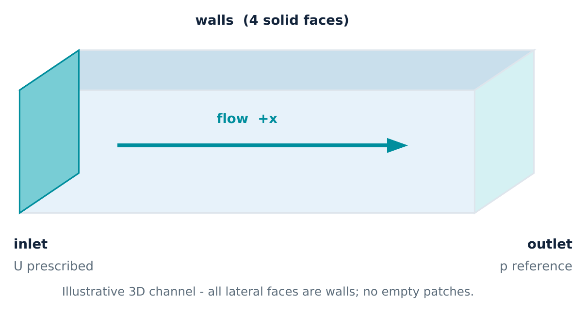
walls, 4 solid faces); there are no empty patches. U is prescribed at the inlet, the p reference is set at the outlet; the flow is along +x.Dimensions of the teaching geometry
| Quantity | Symbol | Demonstration value |
|---|---|---|
| Length | L | 0.100 m |
| Height | H | 0.010 m |
| Width | W | 0.005 m |
| Inlet velocity | Uin | (0.05 0 0) m/s |
| Illustrative viscosity | ν | 1.0 × 10⁻⁶ m²/s |
The mesh boundary names assumed throughout are exactly inlet, outlet, and walls. The four lateral faces belong to the single patch named walls. If your Part 2 geometry uses different names, edit the field files to match your actual mesh.
Optional refresher · Reynolds number
For a rectangular duct, hydraulic diameter Dh = 2HW/(H+W) = 6.67 mm. With the illustrative speed and viscosity, Re = UmeanDh/ν ≈ 333. This is a plausible laminar demonstration; it is not a substitute for validating the real reactor flow.
Deep dive · The channel in numbers: Re, development length and expected pressure drop
The hydraulic diameter comes from the definition Dh = 4A/P (cross-section area over wetted perimeter): A = H·W = 5.0 × 10⁻⁵ m², P = 2(H+W) = 0.030 m, hence Dh = 4·5.0 × 10−5/0.030 = 6.667 × 10⁻³ m. With a uniform inlet the mean velocity equals the imposed one, Umean = 0.05 m/s, and Re = 0.05 · 6.667 × 10−3 / 1.0 × 10−6 = 333.3. Transition in ducts typically occurs above Re ≈ 2000, so the laminar assumption holds with a wide margin.
Development length. A uniform inlet profile is not the developed profile: boundary layers grow from the walls until they fill the section. The classical laminar estimate is Le ≈ 0.05·Re·Dh ≈ 0.05 · 333 · 6.67 mm ≈ 111 mm, i.e. of the same order as the channel length (L = 100 mm, about 15 Dh). The flow is therefore still developing, or only just developed, near the outlet: an important detail when judging the zeroGradient velocity outlet assumption (section 4).
Reference pressure drop. For fully developed flow in a duct with aspect ratio W/H = 0.5, the series solution of the Poisson equation gives f·Re ≈ 62.2 (Darcy friction factor). The kinematic pressure drop over L is Δp/ρ = f (L/Dh) U²/2 = (62.2/333.3) · 15 · (0.05²/2) ≈ 3.5 × 10⁻³ m²/s². The real flow, with its development region, gives a somewhat higher value. It is a useful order of magnitude to compare with the computed p field (which at the inlet will be roughly 0.0035–0.004 m²/s² above the outlet reference).
| Quantity | U = 0.05 m/s | U = 0.06 m/s | U = 0.08 m/s |
|---|---|---|---|
| Flow rate Q = U·A | 2.5 × 10⁻⁶ m³/s | 3.0 × 10⁻⁶ m³/s | 4.0 × 10⁻⁶ m³/s |
| Re | 333 | 400 | 533 |
| Le ≈ 0.05·Re·Dh | ≈ 111 mm | ≈ 133 mm | ≈ 178 mm |
| Developed Δp/ρ over L | ≈ 3.5 × 10⁻³ m²/s² | ≈ 4.2 × 10⁻³ m²/s² | ≈ 5.6 × 10⁻³ m²/s² |
The 0.06 and 0.08 m/s values are used in exercises B and C of section 10. With a water-like ν (ρ ≈ 998 kg/m³), 3.5 × 10⁻³ m²/s² corresponds to about 3.5 Pa.
Deep dive · Which mesh are you using? Part 2 and Appendix A compared
This part quotes the face counts of the 40 × 12 × 8 mesh from Appendix A (coordinates in metres, units [m];). The blockMeshDict built in Part 2 describes the same 100 × 10 × 5 mm channel, but with units [mm]; and a 40 × 10 × 5 division. Geometry and patch names are identical, so the 0/U and 0/p files of this part work unchanged on both; only the numbers read from constant/polyMesh/boundary change.
| Item | Part 2 mesh (40 × 10 × 5) | Appendix A mesh (40 × 12 × 8) |
|---|---|---|
| Cells | 2000 | 3840 |
inlet / outlet faces | 10 × 5 = 50 | 12 × 8 = 96 |
walls faces | 2·(40·5) + 2·(40·10) = 1200 | 2·(40·8) + 2·(40·12) = 1600 |
| Internal faces | 5350 | 10624 |
| Cell size | 2.5 × 1.0 × 1.0 mm | 2.5 × 0.833 × 0.625 mm |
The faces of a patch on a block face are the product of the divisions in the two directions spanning it: the inlet lies in the y–z plane, so it has Ny·Nz faces; the two walls at constant y have Nx·Nz faces each, the two at constant z Nx·Ny. Redoing this count before opening the boundary file is the quickest way to notice a mesh that differs from the expected one.
Boundary-condition map
| Patch | Mesh role | U field | p field |
|---|---|---|---|
inlet | generic patch | fixedValue (0.05 0 0) | zeroGradient |
outlet | generic patch | zeroGradient | fixedValue 0 |
walls | wall | noSlip | zeroGradient |
This is a simple, model-specific configuration: it assumes no gravity/body-force contribution to the pressure equation and no significant reverse flow at the outlet. More general outlet and pressure conditions are discussed later.
Deep dive · Why exactly these assumptions: gravity, backflow and module choice
Gravity. The incompressibleFluid module has no buoyancy term: gravity, if present in a constant-density flow, can be absorbed into a modified pressure and does not affect the velocity field. It matters in variable-density modules, where the solved pressure is p_rgh (pressure minus the hydrostatic contribution ρ g·h) and walls use fixedFluxPressure instead of zeroGradient, precisely because the normal pressure gradient must balance the body forces.
Backflow. With zeroGradient velocity at the outlet, anything entering from outside has no controlled value: if a vortex crosses the outlet the problem becomes ill-posed and the run may diverge. For a straight laminar duct at Re ≈ 333 the flow leaves everywhere and the assumption holds; section 8.3 explains what to do when it does not.
Module. The whole part assumes the incompressibleFluid solver module, selected in system/controlDict with solver incompressibleFluid; and run by foamRun (Part 4). The physical properties (viscosity nu in constant/physicalProperties) and the laminar regime (constant/momentumTransport) are covered in Part 7. The requirements of this module determine which fields are needed in 0/: here only U and p; a turbulence model would add, for example, k, epsilon or omega, and nut.
2. Inside an OpenFOAM field file
Field files live in time directories, normally 0/ at the beginning of a run. The leading zero identifies an initial time, not an input-folder category. Once a solver writes later times, it creates additional directories containing field values.
case/
├── 0/
│   ├── U                  # velocity field
│   └── p                  # kinematic pressure field, for this module
├── constant/
│   └── polyMesh/
│       └── boundary       # mesh patch identities
└── system/
    ├── blockMeshDict
    ├── controlDict
    ├── fvSchemes
    └── fvSolution
Deep dive · Time directories in practice
The name of a time directory is the simulated time value written as a number: 0, 0.01, 0.02 and so on (the format depends on timeFormat and timePrecision in controlDict, Part 4). The solver starts from the directory given by startFrom/startTime: with startTime 0 it reads 0/; with startFrom latestTime it restarts from the last directory written, which contains complete fields and therefore acts as a new initial condition.
The directories written by the solver are not a copy of 0/: internalField usually becomes nonuniform List<vector> with one value per cell, and derived fields appear, such as phi (the volumetric flux on faces, a surfaceScalarField) and the uniform/ subdirectory with time information. Boundary conditions are written back with their type: that is why a restart preserves the patches as they were defined.
Useful tools: foamListTimes lists the time directories excluding 0; foamListTimes -rm deletes them before rerunning from scratch, leaving 0/ untouched. A common tutorial convention is to keep a clean copy of the initial fields (for example 0.orig/) when a pre-processing utility overwrites 0/; with the v14 field functions (section 8.4) that need is reduced.
Three independent declarations
FoamFile: identifies the file object, includingclass,locationandobject.dimensions: declares physical dimensions, checked by OpenFOAM at run time. Foundation v14 supports human-readable names such as[velocity].internalField/boundaryField: specify the initial field in cells and the conditions on the mesh boundary faces.
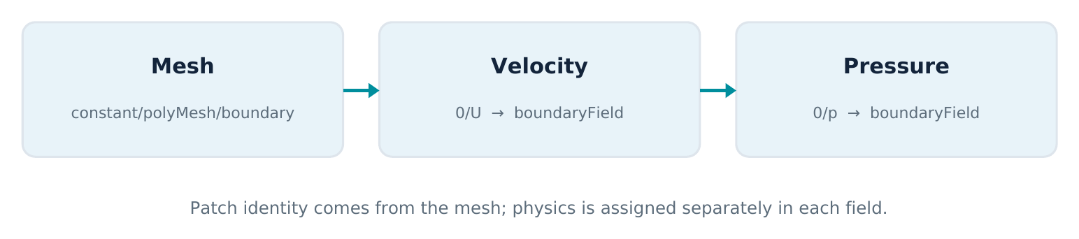
constant/polyMesh/boundary); physics is assigned separately in each field (0/U and 0/p, inside boundaryField).Anatomy of 0/U — illustrative outline
FoamFile
{
    version        2.0;
    format         ascii;
    class          volVectorField;
    location       "0";
    object         U;
}

dimensions         [velocity];
internalField      uniform (0 0 0);
boundaryField
{
    ...
}
Deep dive · The FoamFile header entry by entry
| Entry | Meaning | Notes for v14 |
|---|---|---|
version | I/O format version | Optional; defaults to 2.0. |
format | ascii or binary | Hand-written files are ascii; the solver writes in the format chosen by writeFormat in controlDict. |
class | The C++ type of the object to read | dictionary for dictionaries; for fields volScalarField, volVectorField, volSymmTensorField, volTensorField, surfaceScalarField, pointVectorField… |
location | Path of the file in the case | Optional and informative only; in the initial fields it is "0". |
object | Name of the object | Mandatory according to the guide, although not used; by convention equal to the file name (U, p). |
The vol prefix denotes values at cell centres (plus the values on boundary faces); surface denotes values on faces, point on vertices. The Scalar/Vector part fixes the shape of each value: 1 component for p, 3 for U, 6 for a symmetric tensor, 9 for a general tensor. That is why a wrong class causes read errors of the “vector expected” kind even when the numbers look plausible (section 9).
Deep dive · Named dimensions, exponents and units in v14
Every quantity has a set of seven exponents of the base dimensions, in the order mass, length, time, temperature, amount of substance, current, luminous intensity. The historical numeric form and the named form are equivalent; since v14 the example cases use only named dimensions in input files, and the guide recommends doing so.
| Named form | Numeric form | SI units | Use |
|---|---|---|---|
[velocity] | [0 1 -1 0 0 0 0] | m/s | U |
[kinematicPressure] | [0 2 -2 0 0 0 0] | m²/s² | p in incompressibleFluid |
[pressure] | [1 -1 -2 0 0 0 0] | Pa = kg/(m·s²) | p in compressible modules |
[kinematicViscosity] | [0 2 -1 0 0 0 0] | m²/s | nu |
[length] | [0 1 0 0 0 0 0] | m | coordinates, distances |
Composite expressions are also allowed, such as [sqr(length)/time] or [area/time]. In v14 units are a standard feature: a value can be followed by its unit in square brackets and is converted to base SI units, for example internalField uniform 1 [bar]; (the guide shows exactly this form). Units are checked against the dimensions of the quantity, and according to the v14 release notes dimension checking applies when all geometric fields are read.
To check a name or a conversion, use foamUnits:
foamUnits                      # lists all named dimensions and units
foamUnits velocity             # details of one named dimension
foamUnits kinematicPressure
foamUnits -value "cm/s"        # factor to base units (0.01)
foamUnits -value bar Pa        # factor from the first unit to the second (1e+05)
The exact output depends on the installation; the factor, however, is fixed.
An internal field is not a boundary condition
The internalField initialises values inside the cell volumes. It does not prescribe the inlet, outlet or walls. Those are independently specified inside boundaryField. A zero initial velocity field is compatible with a nonzero imposed inlet velocity.
Optional refresher · Initial value and boundary data
For an unsteady PDE, an initial condition specifies a field throughout the spatial domain at t = t0; a boundary condition constrains its behaviour on ∂Ω. They play different mathematical roles and are not interchangeable.
Deep dive · uniform, nonuniform and what a field really contains
A volVectorField on this mesh contains 3840 internal vectors (one per cell) plus one vector per boundary face: 96 + 96 + 1600 = 1792 patch values. uniform (0 0 0) is shorthand that replicates the same vector in all 3840 cells. The explicit form, which the solver writes in later time directories, is:
internalField   nonuniform List<vector>
3840
(
(0.0498 0.0001 0)
(0.0512 0.0002 0)
...
)
;
The number at the start of the list must equal the number of cells; a mistake here produces a list-size mismatch message. Hand-written files almost always use uniform or, in v14, a field function (section 8.4). Dictionary directives remain available in fields: $internalField expands the value of the internalField entry (useful for instance in value $internalField;), and #include lets you keep the initial values in a shared file.
3. The mesh defines patch identity
After blockMesh, the file constant/polyMesh/boundary lists boundary patches. These entries identify geometry and patch type. They do not, by themselves, prescribe U or p.
Illustrative excerpt of constant/polyMesh/boundary
3
(
     inlet
     {
         type         patch;
         nFaces       96;
         startFace    ...;
     }
     outlet
     {
         type         patch;
         nFaces       96;
         startFace    ...;
     }
     walls
     {
         type         wall;
         nFaces       1600;
         startFace    ...;
     }
)
The counts above correspond to the 40 × 12 × 8 example mesh: 96 inlet faces, 96 outlet faces and 1,600 wall faces. In a real generated boundary file, startFace is a number, not ellipsis; this excerpt is only a reading aid.
Deep dive · The real boundary file and the meaning of startFace
OpenFOAM stores all mesh faces in a single list (constant/polyMesh/faces): first all internal faces, then the boundary faces grouped by patch, one patch after the other. nFaces is how many consecutive faces belong to the patch, startFace is the index (counted from 0) of the first one. For the 40 × 12 × 8 mesh there are 39·12·8 + 40·11·8 + 40·12·7 = 3744 + 3520 + 3360 = 10624 internal faces, so the inlet starts at 10624, the outlet at 10624 + 96 = 10720 and the walls at 10720 + 96 = 10816. The total, 10816 + 1600 = 12416 faces, matches what checkMesh reports. The generated file therefore looks like this:
FoamFile
{
    format      ascii;
    class       polyBoundaryMesh;
    location    "constant/polyMesh";
    object      boundary;
}

3
(
    inlet
    {
        type            patch;
        nFaces          96;
        startFace       10624;
    }
    outlet
    {
        type            patch;
        nFaces          96;
        startFace       10720;
    }
    walls
    {
        type            wall;
        inGroups        List<word> 1(wall);
        nFaces          1600;
        startFace       10816;
    }
)
The line inGroups List<word> 1(wall); (which the generated file shows for patches of type wall) states that the patch belongs to the wall group: every non-generic patch is automatically placed in a group named after its type. This detail becomes relevant in section 9. The patch order is that of the boundary list in blockMeshDict. Never edit nFaces or startFace by hand: they are mesh topology, not parameters.
Name matching
For clarity, we write one explicit boundary condition entry per patch. The patch labels inlet, outlet and walls must be spelled identically in each of 0/U and 0/p. OpenFOAM 14 also supports group and regular-expression selection, but those are not needed yet.
| Boundary file | Field U | Field p |
|---|---|---|
inlet / patch | inlet { type fixedValue; ... } | inlet { type zeroGradient; } |
outlet / patch | outlet { type zeroGradient; } | outlet { type fixedValue; ... } |
walls / wall | walls { type noSlip; } | walls { type zeroGradient; } |
Important · Patch type ≠ field boundary condition
A mesh patch of type wall can carry noSlip for velocity and zeroGradient for pressure. Conversely, constraint types such as symmetry and empty require compatible corresponding field conditions.
Deep dive · Mesh patch types and constraint types
The v14 guide distinguishes three families of mesh patches. Generic patches (patch) typically represent open boundaries such as inlets and outlets and need explicit conditions in every field. Wall patches (wall) also need explicit conditions; the wall type serves models that need to know where walls are (for example wall functions and the wall-distance calculation in turbulence models). The geometric constraints are empty, symmetry, symmetryPlane, wedge, cyclic, cyclicSlip, nonConformalCyclic, nonConformalError, processor, processorCyclic, nonConformalProcessorCyclic and internal: each has a boundary condition of the same name, which is the only one allowed on that patch.
If the field type is not compatible with the constraint (for example zeroGradient on an empty patch), reading stops with an error of the form inconsistent patch and patchField types for patch type empty and patchField type zeroGradient. To avoid rewriting the constraints in every field, the guide suggests including the system file caseDicts/setConstraintTypes, which defines an entry for each constraint group: after the include, only generic and wall patches remain to be configured.
boundaryField
{
    #includeEtc "caseDicts/setConstraintTypes"

    inlet
    {
        type        fixedValue;
        value       uniform (0.05 0 0);
    }
    ...
}
Our channel has no constraint patches, so the include changes nothing here; it becomes convenient in 2D cases (section 8.1) or in cases decomposed for parallel runs, where processor patches appear (see the worked case on MPI parallel execution).
Deep dive · Selection by group and by regular expression
A boundaryField entry can address a patch in three ways, with this precedence: (1) the exact patch name; (2) the name of a group the patch belongs to (for example wall, the automatic group of all patches of type wall); (3) a POSIX regular expression in double quotes, such as ".*Wall" or "(lower|upper)Wall". An exact name always wins over a group or an expression, regardless of order in the file. A compact, fully equivalent version of our 0/p is therefore:
boundaryField
{
    "(inlet|walls)"          // regular expression: double quotes required
    {
        type        zeroGradient;
    }
    outlet                   // exact patch name: highest precedence
    {
        type        fixedValue;
        value       uniform 0;
    }
}
The compact form is useful with dozens of patches, but it makes less obvious which condition each patch receives: that is why this part writes one entry per patch. An important consequence: an entry called wall is not a harmless typo, because it coincides with the group name and therefore applies to all wall patches. If the mesh also has a patch named exactly wall, the entry addresses that one exactly.
4. Write the complete velocity file: 0/U
The velocity is represented by a volVectorField. In Foundation v14, dimensions [velocity] specifies the expected velocity dimensions. The inlet has a fixed uniform velocity in +x.
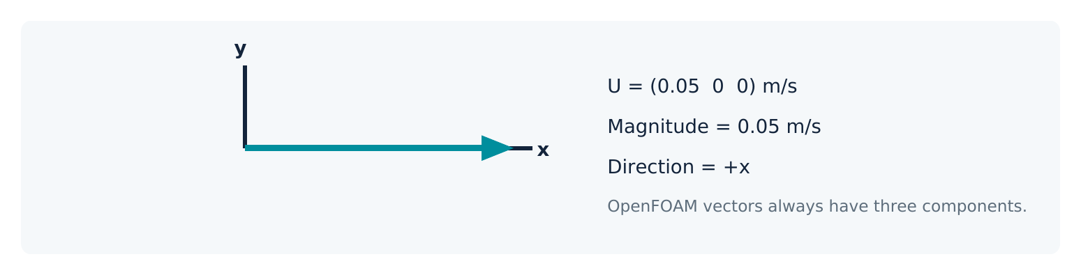
Complete 0/U — reference answer
FoamFile
{
    version        2.0;
    format         ascii;
    class          volVectorField;
    location       "0";
    object         U;
}

dimensions         [velocity];
internalField      uniform (0 0 0);

boundaryField
{
    inlet
    {
        type        fixedValue;
        value       uniform (0.05 0 0);
    }
    outlet
    {
        type        zeroGradient;
    }
    walls
    {
        type        noSlip;
    }
}
Interpret the three patch entries
inlet—fixedValue: all three velocity components are prescribed. Here the vector points along +x.outlet—zeroGradient: the normal gradient of each velocity component is zero. This is a simple outflow approximation, not a general open-boundary model.walls—noSlip: the wall velocity is zero for the fixed, stationary walls of this example.
Notice that noSlip does not need an explicit value entry. By contrast, fixedValue requires its prescribed value.
Deep dive · What fixedValue does at the inlet, in finite-volume terms
In the finite-volume method each cell adjacent to the inlet has a boundary face. fixedValue assigns the vector Ub = (0.05 0 0) m/s to that face. The value enters the equations in two ways: in the convective term, through the volumetric face flux φf = Ub·Sf (Sf is the face area vector, pointing outwards, so here φf < 0: fluid enters); in the diffusive term, through the face-normal gradient, approximated as (Ub − UP)/|d|, where UP is the cell-centre value and |d| the distance between the cell centre and the face centre.
Summing over the 96 inlet faces gives the imposed flow rate: Q = 0.05 m/s × 5.0 × 10⁻⁵ m² = 2.5 × 10⁻⁶ m³/s (2.5 ml/s). With a fixedValue inlet, the flow rate is therefore set exactly by the input, independently of the mesh. The imposed profile is, however, flat (“plug”): next to the walls the velocity jumps from 0.05 m/s to zero within the first cell, and it is the development length estimated in section 1 that rebuilds a realistic profile.
Alternatives for the same inlet, all present in Foundation v14 (check with foamInfo <name>):
flowRateInletVelocity: you impose the (volumetric or mass) flow rate instead of the velocity; the profile on the patch is computed by the condition. Handy when the experimental datum is a flow rate.uniformFixedValue: a uniform value that can vary in time, given byuniformValuefollowed by aFunction1(constant,table,tableFile,sine,square,polynomial,scalewith ramps such aslinearRamp,coded…). Useful for a gradual start-up.functionalFixedValue(new in v14): a non-uniform, and possibly time-varying, value defined by a field function, for example a developed profile (section 8.4).
The worked case on inlet boundary-condition sensitivity compares exactly a flat inlet with a developed profile and measures the downstream consequences.
Deep dive · zeroGradient at the outlet: what it imposes and when it holds
zeroGradient imposes ∂U/∂n = 0. In the discretisation the boundary-face value is simply copied from the adjacent cell centre, Ub = UP, and the diffusive flux through the face is zero. The condition is “natural” if the velocity profile no longer changes along x near the outlet, i.e. if the flow is developed. In our channel the estimated development length (≈ 111 mm) is comparable to the domain length: the x derivatives at the outlet are small but not exactly zero, and the condition introduces a small local error in the last cells. If results near the outlet matter, lengthen the domain downstream.
The outlet flow rate is not imposed by zeroGradient: it is continuity, solved through the pressure equation, that makes it equal to the inlet flow rate. That is why U and p must be thought of as a pair (section 6).
Deep dive · noSlip and the other wall conditions for velocity
noSlip is a condition derived from fixedValue with an implicit zero value: it is equivalent to type fixedValue; value uniform (0 0 0);, but makes the physical intention explicit and needs no value entry. It imposes both zero tangential velocity (adherence) and zero normal velocity (impermeability). It is the condition the v14 guide uses for walls in the tutorials (for example damBreak and the backward-facing step).
| Condition | What it imposes | When to use it |
|---|---|---|
noSlip | U = 0 on the wall | Stationary solid wall (our case) |
movingWallVelocity | Velocity of a moving wall; corrects the flux if the mesh moves | Sliding wall, e.g. the lid of a cavity |
fixedValue | Any vector on the wall | Translating wall with known velocity |
slip | Zero normal component, zero gradient of tangential components | Frictionless wall (idealisation) |
The complete list of conditions available for a vector field is obtained with foamToC -vectorBCs; the description of a single condition, with the example cases that use it, with foamInfo movingWallVelocity.
5. Write the complete pressure file: 0/p
For the selected incompressibleFluid formulation, the primary field p is kinematic pressure, with units m²/s², rather than pressure in pascals. The field class is volScalarField.
Complete 0/p — reference answer
FoamFile
{
    version        2.0;
    format         ascii;
    class          volScalarField;
    location       "0";
    object         p;
}

dimensions         [kinematicPressure];
internalField      uniform 0;

boundaryField
{
    inlet
    {
        type        zeroGradient;
    }
    outlet
    {
        type        fixedValue;
        value       uniform 0;
    }
    walls
    {
        type        zeroGradient;
    }
}
Pressure reference and physical units
The outlet condition fixes a kinematic-pressure reference value. It does not mean the fluid has zero absolute pressure. For constant density ρ, a pressure difference can be converted through ΔpPa = ρ Δpkinematic.
Optional refresher · Pressure gauge and nullspace
In many incompressible formulations only pressure gradients drive the velocity. Without an appropriate reference, the pressure level can be undetermined up to a constant. The outlet fixed value provides a reference for this teaching case. Other formulations may use different reference treatments.
Deep dive · Kinematic pressure: definition and a worked conversion
Dividing the incompressible momentum equation by the constant density ρ gives ∂U/∂t + ∇·(UU) = −∇(p/ρ) + ∇·(ν∇U): the solver works directly with pkin = p/ρ, whose units are Pa/(kg/m³) = m²/s² (equivalent to J/kg, an energy per unit mass). That is why incompressibleFluid requires the kinematic viscosity ν and does not need ρ to solve the flow.
Example. If at steady state the p field is about 0.0035 m²/s² at the inlet and 0 at the outlet (the value estimated in section 1), for water at 20 °C (ρ ≈ 998 kg/m³) the physical pressure drop is ΔpPa = 998 × 0.0035 ≈ 3.5 Pa. The absolute value is obtained by adding the actual outlet pressure, for example atmospheric: pinlet ≈ 101325 + 3.5 Pa. A negative p value inside the domain is therefore not a physical error: it only means a pressure below the reference.
Deep dive · What happens without a fixed value: pRefCell and pRefValue
In the incompressible formulation pressure appears only through its gradient, and the pressure equation built by the solver (a Poisson equation derived from continuity) admits solutions differing by a constant if no patch imposes a value: the matrix is singular, with a nullspace made of constant fields. With fixedValue at the outlet the problem does not arise.
In closed cases, such as a cavity with walls only and therefore zeroGradient everywhere, the level must be set elsewhere: incompressible solvers read from the algorithm dictionary in system/fvSolution (PIMPLE or SIMPLE, Part 6) the entries pRefCell (a cell index) or pRefPoint (a location) and pRefValue (the value assigned there). These entries are used only when no patch fixes the pressure; in our channel they are unnecessary.
Do not mix pressure formulations
| Example model | Possible p representation | Do not assume |
|---|---|---|
| Incompressible single-phase module used here | [kinematicPressure] (m²/s²) | That p = 0 means 0 Pa absolute. |
| Compressible / other physical modules | May use physical pressure [pressure] (Pa) | That you can copy 0/p unchanged between modules. |
For every new solver module, inspect a relevant v14 tutorial and the module documentation before selecting pressure field dimensions or boundary types.
Deep dive · How to check the formulation a module expects
foamInfo incompressibleFluidprints the module description and the example cases that use it.- The v14 guide’s backward-facing step tutorial (
$FOAM_TUTORIALS/incompressibleFluid/pitzDaily) uses exactlydimensions [kinematicPressure];,internalField uniform 0;,zeroGradientat the inlet and walls andfixedValue0 at the outlet: the same structure as this part. - In compressible modules (for example
fluid,shockFluid)pis absolute pressure in Pa with[pressure]and values of the order of 1 bar; in buoyant modulesp_rghalso appears. Copying our0/pinto one of those cases would at best cause a dimension error; at worst, a density computed from a zero absolute pressure. find "$FOAM_TUTORIALS" -path '*/0/p' | headfollowed byfoamDictionary -entry dimensions -value <file>quickly shows which dimensions a module’s tutorials use.
6. What do these conditions mean mathematically?
The syntax only becomes useful when mapped to physical and mathematical constraints. The following simplified descriptions are appropriate for the field and geometry in this unit.
| Boundary type | Simplified meaning | In our case |
|---|---|---|
fixedValue | Dirichlet: the boundary field value is specified. | U at inlet; p at outlet |
zeroGradient | Homogeneous normal-gradient condition: ∂φ/∂n = 0. | U at outlet; p at inlet and walls |
noSlip | For a stationary wall, tangential and normal fluid velocity are zero. | U at walls |
symmetry | Geometric constraint for a true symmetry boundary. | Not used for this 3D channel |
empty | 2D/1D extruded mesh geometric constraint. | Not used for this 3D channel |
Optional refresher · Dirichlet and Neumann
A Dirichlet condition specifies φ on the boundary. A Neumann condition specifies its normal derivative. A finite-volume boundary condition must be interpreted alongside the governing equation, discretisation and physical assumptions; syntax alone does not guarantee a well-posed CFD model.
Deep dive · The v14 basic conditions and their discrete form
The v14 guide lists six basic conditions (sources in $FOAM_SRC/finiteVolume/fields/fvPatchFields/basic), from which almost all the others derive. Writing φP for the adjacent cell-centre value, φb for the boundary-face value and Δ = 1/|d| for the inverse distance between the two points:
| Condition | Required entries | Face value | Face normal gradient |
|---|---|---|---|
fixedValue | value | φb = φref | Δ(φb − φP) |
fixedGradient | gradient | φb = φP + g/Δ | g |
zeroGradient | none | φb = φP | 0 |
calculated | value | computed from other fields | — |
mixed | refValue, refGradient, valueFraction | w φref + (1 − w)(φP + gref/Δ) | blend of the two |
directionMixed | as mixed, with a tensorial valueFraction | fixed value in some directions, gradient in the others | — |
With valueFraction w = 1 the mixed condition becomes a fixed value, with w = 0 a fixed gradient. The most common derived conditions are built this way: inletOutlet, for instance, is a mixed condition that switches to a fixed value where the flow enters and to zero gradient where it leaves. In the linear-system matrix each condition contributes a coefficient on the diagonal of the adjacent cell and a source term: fixedValue adds both (the imposed value is a source, the dependence on φP strengthens the diagonal), zeroGradient adds neither in the diffusive term.
Why are U and p treated as a pair?
For incompressible flow, velocity and pressure are coupled through momentum and continuity. Specifying an inlet velocity and an outlet pressure reference is one common simple pairing. It is not universally appropriate for flow reversal, imposed flow rate, moving walls, buoyant flow or compressible models.
Deep dive · Why the pairing works: counting the information
The equations are ∇·U = 0 and ∂U/∂t + ∇·(UU) = −∇p + ν∇²U. Velocity satisfies a transport-diffusion equation that requires either the value or the normal gradient on every boundary; pressure has no evolution equation of its own: in the SIMPLE/PIMPLE algorithm it satisfies a Poisson equation built by enforcing continuity on the corrected fluxes. Two practical rules follow.
- Where U is imposed, p takes zero gradient. At the inlet and walls the flux through the face is already fixed by the velocity; the pressure equation must not correct it, and the consistent condition is a normal gradient (zero, without body forces). This is exactly the choice of this part.
- Where p is imposed, U takes zero gradient. At the outlet the pressure fixes the level and the velocity adapts, so that the outflow rate follows from continuity. Imposing both U and p on the same boundary over-determines the problem; imposing neither anywhere leaves it undetermined.
On walls, strictly speaking, the normal pressure gradient is tied to the viscous terms (∂p/∂n = ν∇²U·n); zeroGradient is the standard approximation, accurate for flows like this one. With body forces, fixedFluxPressure is used, which computes the gradient consistent with the imposed flux.
Initialisation affects convergence, not the prescribed boundary
The initial field U = (0 0 0) in every cell is a valid simple starting guess even though the inlet already imposes U = (0.05 0 0). A different initial guess can change the convergence history; it does not replace the boundary condition.
Deep dive · What happens at the first step with zero initial U
At the first step the internal field is at rest and only the inlet faces have non-zero velocity: the inflow, 2.5 × 10⁻⁶ m³/s, has no matching outflow. The first pressure correction solves the Poisson equation and redistributes velocity over the whole domain, so that continuity is satisfied immediately: in an incompressible fluid pressure information propagates instantaneously. That is why, in the log, the initial residuals of the first steps are high (often close to 1) and then decrease.
Starting from uniform (0.05 0 0) throughout reduces the initial transient; starting from a developed field (for example from a previous run, mapped with mapFields) reduces it further. For a steady calculation the final result does not change; for a physically transient calculation, however, the initial field is part of the problem and must be chosen as carefully as the boundary conditions.
7. Practical laboratory: assemble and inspect
Work only in your editable copy of the channel case. Keep the original Part 2 mesh and any existing validated solver controls. The purpose of this exercise is to add or modify field files; do not change the OpenFOAM installation.
Stage 1 — Confirm the mesh
foamVersion
cd /path/to/your/editable/channelCase
blockMesh
checkMesh
sed -n '1,180p' constant/polyMesh/boundary
Read the patch count and patch names from the generated boundary file. If these are not exactly inlet, outlet, and walls, you must adapt the examples accordingly. Never rename a mesh patch solely in a field file.
Deep dive · What checkMesh should report for the Appendix A mesh
Predicting the numbers before running is the most effective way to verify. For the 40 × 12 × 8 mesh of Appendix A the expected values are:
| checkMesh item | Expected value | Where it comes from |
|---|---|---|
| points | 4797 | 41 × 13 × 9 |
| faces | 12416 | 10624 internal + 1792 boundary |
| internal faces | 10624 | 39·12·8 + 40·11·8 + 40·12·7 |
| cells / hexahedra | 3840 / 3840 | 40 × 12 × 8 |
patch inlet: faces, points | 96, 117 | 12 × 8; 13 × 9 |
patch outlet: faces, points | 96, 117 | 12 × 8; 13 × 9 |
patch walls: faces, points | 1600, 1640 | 1794 boundary points minus the 2 × 77 interior to inlet and outlet |
| bounding box | (0 0 0) (0.1 0.01 0.005) | vertices, in metres |
The last line must be Mesh OK. The cells measure 2.5 × 0.833 × 0.625 mm, so the reported maximum aspect ratio will be of the order of 4, entirely acceptable. For the Part 2 mesh (40 × 10 × 5) the numbers change as shown in section 1. sed -n '1,180p' prints the first 180 lines of the file, more than enough for a three-patch boundary file; checkMesh also reports the same names in its patch table.
Stage 2 — Write the field files
mkdir -p 0
# Open 0/U and 0/p in your preferred text editor.
# Insert the complete examples from Sections 4 and 5.
Check the class, object, named dimensions, every brace and every semicolon. The field files are ASCII/UTF-8 text; indentation improves readability but is not part of the syntax.
Deep dive · Writing the files without an editor and without copy errors
If you prefer not to use an interactive editor, a shell here-document writes the file exactly as pasted; the quotes around EOF stop the shell from expanding $ and other special characters:
cat > 0/p <<'EOF'
FoamFile
{
    format      ascii;
    class       volScalarField;
    object      p;
}
dimensions      [kinematicPressure];
internalField   uniform 0;
boundaryField
{
    inlet  { type zeroGradient; }
    outlet { type fixedValue; value uniform 0; }
    walls  { type zeroGradient; }
}
EOF
The example also shows that the multi-line layout is only a convention: inlet { type zeroGradient; } on one line is identical to the expanded form. Beware of invisible characters when copying from PDFs or web pages: typographic quotes (“ ”) instead of ", long dashes instead of the minus sign, non-breaking spaces. The OpenFOAM parser does not recognise them and the reported error can look incomprehensible. A quick check: grep -nP '[^\x00-\x7F]' 0/U 0/p lists the lines with non-ASCII characters.
Stage 3 — Inspect entries structurally
foamDictionary 0/U
foamDictionary -entry dimensions -value 0/U
foamDictionary -entry internalField 0/U
foamDictionary -entry 'boundaryField/inlet' 0/U
foamDictionary -entry 'boundaryField/outlet/type' -value 0/p
foamDictionary -entry 'boundaryField/walls/type' -value 0/U
The nested path syntax for foamDictionary uses /. Successful extraction of an entry verifies that the file can be parsed as a dictionary; it does not prove that all model-specific conditions are physically correct.
Deep dive · The expected foamDictionary output and three more commands
The first command prints the whole file without comments. The others should produce output like this (exact spacing may differ):
$ foamDictionary -entry dimensions -value 0/U
[velocity]
$ foamDictionary -entry internalField 0/U
internalField   uniform (0 0 0);
$ foamDictionary -entry 'boundaryField/inlet' 0/U
inlet
{
    type            fixedValue;
    value           uniform (0.05 0 0);
}
$ foamDictionary -entry 'boundaryField/outlet/type' -value 0/p
fixedValue
$ foamDictionary -entry 'boundaryField/walls/type' -value 0/U
noSlip
-value prints only the data, without keyword and semicolon: the form suited to scripts. Three more useful commands: -keywords lists the keys of a sub-dictionary and so checks patch coverage at once; -set changes an entry without opening the editor (here, ready for exercise B of section 10):
foamDictionary -entry boundaryField -keywords 0/U
foamDictionary -entry boundaryField -keywords 0/p
foamDictionary -entry boundaryField/inlet/value -set "uniform (0.08 0 0)" 0/U
The first two must print inlet, outlet and walls, the same names as in the boundary file. If an entry does not exist, foamDictionary stops with an error naming the missing key and the dictionary path: that is already a first consistency check.
Stage 4 — Validate with the existing solver setup
If the case already has a valid constant/ physics configuration and system/controlDict, fvSchemes and fvSolution, run the established foamRun workflow. Otherwise stop here: later parts (4, 5, 6 and 7) explain the missing dictionaries.
# Only if the complete case has already been configured:
foamRun > log.foamRun 2>&1
# Then inspect the log in a separate step:
less log.foamRun
Important · Mesh checks do not validate boundary conditionscheckMesh validates mesh topology and quality. It cannot certify that a pressure outlet is physically meaningful or that a velocity condition is suitable for a given flow.
Deep dive · Reading the log for field errors
Field-file errors appear early in the log, right after the mesh is created, when the module reads the fields (lines such as Reading field p and Reading field U). A fatal read error begins with --> FOAM FATAL IO ERROR, gives a message, then the file and line number (file: .../0/U/boundaryField/walls at line 31. or similar), and ends with FOAM exiting. Since the log can be long, search for it directly:
grep -n "FOAM FATAL" log.foamRun
grep -n -A 12 "FOAM FATAL" log.foamRun | head -40
If the run starts, the first physical checks are continuity (the continuity errors reported at each step must stay small) and the outlet flow rate, which must tend to 2.5 × 10⁻⁶ m³/s. Post-processing the flow rate on a patch is covered in the worked cases, for example the laminar channel with Poiseuille validation.
8. Special cases you will encounter
8.1 Two-dimensional simulations
A standard OpenFOAM 2D calculation is represented by an extruded one-cell-thick mesh with the front/back faces assigned the geometric constraint empty. In each required field, those patches also use type empty;. Do not set empty on a physical 3D wall just because you do not want flow through it.
Field boundary condition for an actual empty mesh patch
frontAndBack
{
    type empty;
}
Deep dive · Turning the channel into a 2D case, and what changes in the physics
To obtain a 2D version of our channel in the x–y plane, two changes to blockMeshDict suffice: one cell in z, i.e. (40 12 1), and the two constant-z faces, (0 3 2 1) and (4 5 6 7), moved from walls to a new patch frontAndBack of type empty. Then, in every field, add the entry frontAndBack { type empty; } (or include caseDicts/setConstraintTypes). The empty direction is not solved: checkMesh shows it by reporting two geometric directions instead of three.
The physics, however, changes: the 2D case represents a channel between two parallel flat plates, infinitely wide in z, no longer a rectangular duct. The hydraulic diameter becomes 2H = 20 mm, Re at the same speed triples (≈ 1000) and the developed profile is the plane Poiseuille parabola, with peak velocity 1.5 times the mean. This is the case treated in the first worked case, laminar flow between flat plates and Poiseuille validation. Typical mistakes: forgetting the empty patch in just one field (missing-entry error for frontAndBack), using more than one cell in the empty direction, or using zeroGradient on an empty patch (inconsistent patch types error, section 3).
For axisymmetric cases a thin wedge mesh is used instead, with two patches of type wedge and the corresponding wedge field condition.
8.2 Symmetry is not a frictionless wall
Use symmetry only where the physical problem and geometry justify reflection symmetry. It restricts the solution in a specific way; it is not interchangeable with noSlip or a generic open boundary.
Deep dive · What symmetry imposes and an example on our channel
On a symmetry plane the normal velocity component is zero, the tangential components have zero normal gradient and scalars (such as p) have zero normal gradient: the solution mirrors itself across the plane. Mathematically, on a flat face the result coincides with that of the slip velocity condition, which is why one hears “frictionless wall”; but the meaning is different: symmetry states that the same reflected solution lies on the other side, so perturbations (vortices, instabilities) are also forced to be symmetric. symmetryPlane requires a perfectly planar patch; symmetry also accepts patches that are not perfectly planar.
Example: our duct is symmetric about the plane z = 2.5 mm. One could model half the section (z from 0 to 2.5 mm, 4 cells in z) with the z = 2.5 mm face of type symmetry in the mesh and symmetry in every field, halving the cell count. This is legitimate only because geometry, boundary conditions and steady laminar flow are all symmetric; for a flow with unsteady separation it would not be. Here too the types must agree: symmetry in the mesh and symmetry in the field.
8.3 Reverse flow at an outlet
The simple zeroGradient velocity outlet is not robust for every configuration. If backflow is expected, investigate outlet-specific conditions such as pressureInletOutletVelocity and appropriate pressure conditions using the official documentation and tutorials. Choosing a backflow condition is a physical modelling decision, not a mechanical replacement.
Deep dive · The v14 outlet conditions for backflow
| Condition | Field | Behaviour | Entries |
|---|---|---|---|
inletOutlet | scalars and vectors | Zero gradient where fluid leaves, fixed value where it enters | inletValue |
pressureInletOutletVelocity | U | Zero gradient, except the tangential component, fixed for inflow | optional tangentialVelocity (default 0; in v14 also a field function) |
totalPressure | p | p = p0 on outflow; on subsonic inflow p = p0 minus the dynamic pressure | p0 |
entrainmentPressure | p | Like totalPressure, but the inflow term uses the normal velocity component; the guide considers it more robust | p0 |
prghTotalPressure | p_rgh | Counterpart of totalPressure for buoyant modules | p0 |
The typical pairing for an open boundary where flow may enter or leave is pressureInletOutletVelocity on U with totalPressure (or entrainmentPressure) on p, as on the atmosphere patch of the guide’s damBreak tutorial. To find out whether backflow actually occurs, check the sign of the flux on the outlet patch: local negative values of phi on the outlet indicate fluid re-entering. v14 also introduces, as a prototype, meanInletOutlet, a scalar variant of inletOutlet in which the inflow value is the mean of the adjacent cell values.
8.4 New in OpenFOAM 14: field functions
Foundation v14 introduces field functions that can initialise non-uniform internal fields directly. This can remove the need for a separate initialisation utility in appropriate cases. It is an advanced preview, not a requirement of the current reference case.
Conceptual extract from the official shock-tube field-function example
internalField
{
    type           zonal;
    defaultValue 1 [bar];
    zones
    {
         lowPressure
         {
             type box;
             box   (0 -1 -1) (5 1 1);
             value 0.1 [bar];
         }
    }
}
This is a separate pressure-model example, not a replacement for our channel 0/p (which uses kinematic pressure). The v14 functionalFixedValue boundary condition similarly allows values based on field functions.
Optional refresher · Nonuniform fielduniform denotes one value applied everywhere in the relevant field region. nonuniform typically supplies values per cell or face. v14 field functions provide a third, higher-level way to initialise distributions from geometric or functional rules.
Deep dive · How to read the zonal example
The example comes from the $FOAM_TUTORIALS/shockFluid/shockTube tutorial, a 1D compressible case. internalField is no longer a value but a sub-dictionary with a type: zonal assigns different values in different mesh zones. defaultValue 1 [bar] applies everywhere outside the zones; here the [bar] unit is converted to 105 Pa, consistent with the [pressure] dimensions of that field. The lowPressure zone is generated on the fly as a cell zone by a box generator (the cells whose centre lies in the box with corners (0 −1 −1) and (5 1 1), in metres), and there the value is 0.1 [bar]. The result is the classic initial pressure jump of the Riemann problem.
Before v14 the same result required a uniform field in 0/, a backup copy and running setFields with a setFieldsDict; now the definition lives in the field file itself and is reproducible without extra steps. setFields still exists in v14.
Deep dive · The field-function types and functionalFixedValue
| Type | What it does (v14 guide, §6.1) |
|---|---|
zonal | Different values in different mesh zones, with a default elsewhere. |
surfaces | Regions separated by surfaces (searchable surfaces, STL/OBJ files); cut cells receive fractional values, hence a smoother interface. |
coded | Values defined by code compiled on the fly, in an evaluate block (and update for time updates), with the references field, C (cell centres) and t (time). |
distanceFunction | A Function1 of position along a given direction. |
fieldFunction | A Function1 of another field, for example a property as a function of temperature. |
timeFunction | A Function1 of time only. |
There are also applied field functions that replace older utilities: atmosphericBoundaryLayerVelocity and the corresponding ones for k and epsilon (instead of setAtmBoundaryLayer), waveAlpha and waveVelocity (instead of setWaves). The guide’s coded example, a swirling flow, has this structure:
internalField
{
    type            coded;
    evaluate
    #{
        field = velocity(1, 0, 0) + (C ^ rate(2, 0, 0));
    #};
}
Here velocity(1, 0, 0) is a vector with velocity dimensions and C ^ rate(2, 0, 0) the cross product of the cell-centre position and an angular rate: a translation plus a rigid rotation. The same distribution is carried onto a patch with functionalFixedValue, which reuses the internal-field definition through the $internalField macro:
inlet
{
    type            functionalFixedValue;
    value           $internalField;
}
According to the release notes, functionalFixedValue initially supports the zonal, distanceFunction and coded functions. A natural application to our channel would be a developed inlet profile instead of the flat one: for example the product-of-parabolas approximation u(y,z) = 2.25 Umean (1 − (2y′/H)²)(1 − (2z′/W)²), with y′ and z′ measured from the section centre, has exactly the mean Umean (each parabola averages 2/3, and 2.25 × 4/9 = 1). Before writing it in a real case, compare the syntax with the v14 guide example (§6.1 and §6.5) and with foamInfo functionalFixedValue.
9. Troubleshooting: diagnose the first real error
When OpenFOAM reports a field-read error, focus on the first informative error message, its file path and the offending dictionary entry. Correct one cause at a time.
| Symptom | Probable cause | First check |
|---|---|---|
| Patch entry is missing | A mesh patch has no matching field condition. | Compare polyMesh/boundary with boundaryField. |
| Unknown patch-field type | Typo or model-specific BC unavailable. | Check type, foamInfo and available BCs. |
| Wrong dimensions | The field dimensions do not match what the model expects. | Check named dimensions and module. |
| Expected vector / scalar | Value shape or field class is wrong. | Check volVectorField vs volScalarField. |
| Parser stops at a later line | Missing semicolon or brace earlier in the file. | Inspect the whole surrounding block. |
| Case runs but physically wrong | Wrong BC selection, direction, geometry or pressure interpretation. | Revisit the physics, not just the syntax. |
Deep dive · What these errors look like in the log
The exact text depends on the version and on where the error is detected, but the following patterns are typical of the Foundation line. Recognising them saves a lot of time:
| Symptom | Typical message pattern | What to read |
|---|---|---|
| Missing patch entry | Cannot find patchField entry for walls | The missing patch name and the file (0/U or 0/p) |
| Unknown type | Unknown patchField type noslip for patch walls | The list of valid types follows: look for the right name (here noSlip, capital S) |
Missing value | keyword value is undefined in dictionary .../0/U/boundaryField/inlet | The path names the exact patch |
| Vector expected | Expected a '(' while reading VectorSpace…, e.g. with value uniform 0.05; in 0/U | The reported line contains a scalar where a vector is needed |
| Inconsistent constraint | inconsistent patch and patchField types for patch type empty and patchField type zeroGradient | The type in the mesh and the type in the field |
| Dimensions | messages about different or incompatible dimensions, with the two exponent sets printed | Compare the exponents with foamUnits |
Every fatal error also reports file: … with the sub-dictionary path and a line number. For syntax errors (semicolons, braces) the reported line is where the parser noticed the problem, often well after the cause.
Use the documentation tools
foamInfo fixedValue
foamInfo noSlip
foamInfo zeroGradient
foamToC -scalarBCs
foamToC -vectorBCs
foamUnits velocity
foamUnits kinematicPressure
In v14, foamInfo explains the model/condition where available, foamToC lists compiled run-time selection options, and foamUnits provides information about named dimensions and units. Their outputs depend on the installed libraries and environment.
Deep dive · What to expect from foamInfo, foamToC and foamUnits
foamInfo noSlipprints the documented header of the condition’s source (description, usage with an example entry) and the list of tutorials that use it: a quick way to find a working example to study.foamToC -scalarBCsandfoamToC -vectorBCsinterrogate the compiled libraries directly and produce long lists; filter them, for examplefoamToC -vectorBCs | grep -i slip.foamToCoutput is more definitive thanfoamInfo, because it reflects what is actually loadable.foamToC -search noSlipreports which selection table contains an entry;-solver incompressibleFluidloads that module’s libraries before listing.foamUnits velocityandfoamUnits kinematicPressureshow the corresponding exponents ([0 1 −1 0 0 0 0] and [0 2 −2 0 0 0 0]) and associated units; with no argument,foamUnitslists all defined named dimensions and units.
Three controlled fault exercises
- Error A: change
wallstowallonly in0/U. Predict what will no longer match. Restore it. - Error B: remove the semicolon after
dimensions [velocity]. Check whether dictionary parsing fails; restore the file. - Error C: set
0/pto[velocity]. Explain why the units contradict the field meaning. Restore it.
For each fault record: expected problem, observed message, source file, minimal correction. Do not edit production or shared research cases.
Deep dive · What really happens in the three faults
Error A — beware of the wall group. The intuitive prediction is that the walls patch is left without an entry in 0/U and that reading stops with Cannot find patchField entry for walls. In OpenFOAM 14, however, every patch of type wall automatically belongs to the wall group (section 3), and an entry called wall in boundaryField is interpreted as a group selection: the walls patch still receives noSlip and the case is, in all likelihood, read without errors. It is a useful lesson: a “wrong” name can be a valid name with a different meaning. To actually see the missing-entry error, use a name that matches no group, for example wals. Try both variants and record what happens.
Error B — parsing does not necessarily fail. A primitive entry extends to the first ;: without the semicolon, the dimensions entry also swallows the next line and becomes [velocity] internalField uniform (0 0 0), while the internalField key disappears. The file remains a syntactically readable dictionary, so foamDictionary 0/U may work; the fault shows with foamDictionary -entry dimensions -value 0/U (which also prints the rest of the line) and with foamDictionary -entry internalField 0/U, which fails because the key no longer exists. The solver will stop with an error about the dimensions entry or about the missing internalField: either way, the reported line is not the one with the missing semicolon.
Error C — dimensions. Kinematic pressure has dimensions [0 2 −2 0 0 0 0] (m²/s²), velocity [0 1 −1 0 0 0 0] (m/s): the ∇p term of the momentum equation must have the dimensions of an acceleration (m/s²), and with p in m/s it would have dimensions 1/s. OpenFOAM checks dimensional consistency: according to the release notes, in v14 the check happens when the fields are read, otherwise at the first operation combining incompatible terms. The message prints the two exponent sets; the file to correct is 0/p.
| Fault | Expected problem | Observed message | Source file | Minimal correction |
|---|---|---|---|---|
| A | … | … | 0/U | wall → walls |
| B | … | … | 0/U | add ; |
| C | … | … | 0/p | [velocity] → [kinematicPressure] |
The table is a logbook template: fill the empty columns with your predictions and the messages you actually observe.
10. Exercises and assessment
Exercise A — Read and classify (guided)
Without running the solver, use the complete U and p examples and answer:
- Which file contains a vector field? How do you know?
- Which entry describes values inside cells? Which entries describe patches?
- Why can
internalField uniform (0 0 0)coexist with an inlet velocity of 0.05 m/s? - Where is the pressure reference defined?
- Which three identifiers must match the mesh boundary file?
Worked solution · Exercise A
0/U: as shown byclass volVectorFieldin the header, the[velocity]dimensions and the shape of the values, always in parentheses with three components.0/pis avolScalarFieldwith one-component values.internalFielddescribes the cell values; the entries insideboundaryField(inlet,outlet,walls) describe the patches.- Because the internal value is only the initial condition (a starting guess), while the inlet velocity is a boundary condition imposed on the faces of the
inletpatch for the whole run; the two data play different mathematical roles (sections 2 and 6). - In
0/p, on theoutletpatch:type fixedValue; value uniform 0;. inlet,outletandwalls, spelled identically in both files.
Exercise B — Modify and predict (partly guided)
Change the prescribed inlet velocity to (0.08 0 0) m/s. Before executing anything, state:
- Which exact file, entry and component must change?
- What is the new mean volumetric inflow for a uniform inlet if the inlet area is 0.010 × 0.005 m²?
- Does the initial internal value also have to be changed?
- Why would a new velocity magnitude demand renewed reflection on Reynolds number and regime?
Checkpoint for exercise B
For a uniform normal inlet velocity of 0.08 m/s and area of 5.0 × 10⁻⁵ m²: Q = U A = 4.0 × 10⁻⁶ m³/s. A changed internal initial guess is optional; the inlet boundary value is the prescribed flow input.
Worked solution · Exercise B
- File
0/U, entryboundaryField/inlet/value, x component:uniform (0.05 0 0)becomesuniform (0.08 0 0). In one command:foamDictionary -entry boundaryField/inlet/value -set "uniform (0.08 0 0)" 0/U.0/pdoes not change. - Q = 0.08 × (0.010 × 0.005) = 0.08 × 5.0 × 10−5 = 4.0 × 10⁻⁶ m³/s (4 ml/s), as in the checkpoint.
- No.
uniform (0 0 0)remains a valid initial guess; it can be set to(0.08 0 0)to shorten the transient, but the steady result does not change. - Because Re = U Dh/ν grows proportionally: from ≈ 333 to ≈ 533. The regime remains laminar, but the estimated development length rises to ≈ 178 mm, almost twice the channel: the
zeroGradientoutlet assumption becomes less accurate, the pressure drop grows (≈ 5.6 × 10⁻³ m²/s² over the developed length) and, with a fixed time step, the Courant number increases by 60 % (Part 4). More generally, every change of velocity should prompt a check that the model assumptions (laminar, no backflow) still hold.
Exercise C — Build independently (unguided)
Starting from a valid channel mesh whose patches are named inlet, outlet and walls, write 0/U and 0/p from an empty 0/ directory. Requirements:
- Laminar incompressible flow along +x, with U at inlet = 0.06 m/s.
- No-slip on all solid duct faces.
- A simple outlet kinematic-pressure reference of 0.
- Uniform zero initial U and p fields.
- Every mesh patch explicitly covered in both field files.
Acceptance checklist
| Check | Evidence expected |
|---|---|
| Structure | Both field files contain a valid FoamFile header and the required field keys. |
| Types | U is volVectorField; p is volScalarField. |
| Dimensions | Named dimensions match the selected incompressible formulation. |
| Patch coverage | All three mesh patch names appear in both boundaryField dictionaries. |
| Physics | The field conditions are consistent with the stated idealised channel problem. |
| Interpretation | You can explain every boundary entry without reference to an answer sheet. |
The goal is not to obtain a particular pressure-drop curve yet. This part assesses configuration literacy, not full research-model validation.
Reference solution · Exercise C, with the checklist verifications
0/U:
FoamFile
{
    version        2.0;
    format         ascii;
    class          volVectorField;
    location       "0";
    object         U;
}

dimensions         [velocity];
internalField      uniform (0 0 0);

boundaryField
{
    inlet
    {
        type        fixedValue;
        value       uniform (0.06 0 0);
    }
    outlet
    {
        type        zeroGradient;
    }
    walls
    {
        type        noSlip;
    }
}
0/p is identical to the one in section 5: [kinematicPressure], uniform 0, zeroGradient on inlet and walls, fixedValue with uniform 0 on outlet. Control quantities: Q = 0.06 × 5.0 × 10−5 = 3.0 × 10⁻⁶ m³/s, Re ≈ 400, development length ≈ 133 mm, developed Δp/ρ ≈ 4.2 × 10⁻³ m²/s².
Each row of the acceptance checklist has a command that produces the evidence:
foamDictionary -entry FoamFile/class -value 0/U         # volVectorField
foamDictionary -entry FoamFile/class -value 0/p         # volScalarField
foamDictionary -entry dimensions -value 0/U             # [velocity]
foamDictionary -entry dimensions -value 0/p             # [kinematicPressure]
foamDictionary -entry boundaryField -keywords 0/U       # inlet outlet walls
foamDictionary -entry boundaryField -keywords 0/p       # inlet outlet walls
foamDictionary -entry boundaryField/inlet/value -value 0/U   # uniform (0.06 0 0)
The “Physics” and “Interpretation” rows have no command: they are verified by explaining aloud, patch by patch, why each condition is the right one, with the arguments of sections 4–6.
Appendix A. Minimal reference mesh for an independent test
If Part 2 did not leave a compatible mesh, the following single-block 3D system/blockMeshDict creates the exact patch names used throughout this part. All coordinates are in metres.
FoamFile
{
    version        2.0;
    format         ascii;
    class          dictionary;
    location       "system";
    object         blockMeshDict;
}

units   [m];

vertices
(
    (0     0         0)        // 0
    (0.100 0         0)        // 1
    (0.100 0.010     0)        // 2
    (0     0.010     0)        // 3
    (0     0         0.005)    // 4
    (0.100 0         0.005)    // 5
    (0.100 0.010     0.005)    // 6
    (0     0.010     0.005)    // 7
);

blocks
(
    hex (0 1 2 3 4 5 6 7) (40 12 8) simpleGrading (1 1 1)
);

edges ();

boundary
(
    inlet
    {
        type patch;
        faces ((0 4 7 3));
    }
    outlet
    {
        type patch;
        faces ((1 2 6 5));
    }
    walls
    {
        type wall;
        faces
        (
            (0 1 5 4)
            (3 7 6 2)
            (0 3 2 1)
            (4 5 6 7)
        );
    }
);

mergePatchPairs ();
The mesh contains 40 × 12 × 8 = 3,840 hexahedral cells. The four long faces share the patch walls. This mesh definition is sufficient for blockMesh and checkMesh; it is not a complete runnable CFD case without the remaining solver dictionaries and properties.
Deep dive · Checking face orientation and the bare minimum for blockMesh
Every boundary face must be listed so that, applying the right-hand rule to the vertex order, the normal points out of the block. For the inlet (0 4 7 3): 0→4 is +z, 4→7 is +y, and z × y = −x, outwards on the x = 0 plane. For the outlet (1 2 6 5): +y then +z, y × z = +x. For the walls: (0 1 5 4) gives −y, (3 7 6 2) gives +y, (0 3 2 1) gives −z, (4 5 6 7) gives +z. All point outwards, and the block hex (0 1 2 3 4 5 6 7) is right-handed (face 0-1-2-3 traversed anticlockwise seen from +z, with 4-5-6-7 above it). blockMesh reports wrongly oriented faces; checkMesh detects them as open boundary faces or negative volumes.
units [m]; is the blockMesh units control introduced in v14 (Part 2 uses units [mm]; with coordinates in millimetres; both forms replace the old scale). Running blockMesh also requires a minimal system/controlDict and the constant/ directory; the full mesh-only sequence is in Part 2. Resulting cells: 2.5 mm in x, 0.833 mm in y, 0.625 mm in z.
Appendix B. Key interpretation table
| Entry | Meaning | Example in this part |
|---|---|---|
FoamFile.class | Type of object to read | volVectorField for U |
FoamFile.object | Field object name | U or p |
dimensions | Physical dimensions | [velocity] |
internalField | Values initially in cells | uniform (0 0 0) |
boundaryField | Patch-specific conditions | inlet, outlet, walls |
type fixedValue | Prescribed field value | U at inlet |
type zeroGradient | Zero normal gradient | p at inlet |
type noSlip | Zero wall velocity | U on stationary walls |
Appendix C. Sources and further reading
All syntax and v14-specific features in this part are based on the OpenFOAM Foundation / CFD Direct v14 User Guide. The documentation for OpenFOAM.com releases belongs to a separate distribution and should not be substituted without checking compatibility.
- User Guide overview —
doc.cfd.direct/openfoam/user-guide-v14/ - 4.2 Input/output file format —
doc.cfd.direct/openfoam/user-guide-v14/basic-file-format - 5.4 blockMesh —
doc.cfd.direct/openfoam/user-guide-v14/blockmesh - 6.1 Field functions —
doc.cfd.direct/openfoam/user-guide-v14/field-functions - 6.3 Introduction to boundary conditions —
doc.cfd.direct/openfoam/user-guide-v14/boundary-conditions - 6.4 Derived boundary conditions —
doc.cfd.direct/openfoam/user-guide-v14/derived-boundary-conditions - 4.7 Case-management tools —
doc.cfd.direct/openfoam/user-guide-v14/case-management - OpenFOAM 14 release notes —
openfoam.org/release/14/
v14 guide pages cited in the deep dives:
- 5.3 Mesh boundary (patch types, groups)
- 6.2 Field sources (the optional
sourcesentry of field files) - 6.5 Field functions in boundary conditions (
functionalFixedValue) - 2.1 Backward-facing step (
incompressibleFluidtutorial with[kinematicPressure])
Deep dive · The optional sources entry in field files
Besides dimensions, internalField and boundaryField, the v14 guide lists a fourth, optional field-file entry: sources. It is needed when a source model in constant/fvModels introduces fluid inside the domain (for example a volumeSource): the field must know the value carried by the injected fluid, for instance its velocity. sources is a dictionary with one entry per source, named like the model in fvModels, and each entry uses a condition such as uniformFixedValue with uniformValue. Our channel has no internal sources, so the entry is absent; it is useful to recognise it when you meet it in a tutorial.
Next unit · Part 4 — controlDict and simulation control
You have now defined which fields exist and what happens at their boundaries. The next part explains how OpenFOAM starts, advances and writes a simulation, and how those settings appear in system/controlDict.
Next part: OpenFOAM 14 Part 4: controlDict and Simulation Control. Back to the Learning OpenFOAM 14 project index.