

The 2D21 Thyratron: From Historical Curves to SPICE Models
10. Zabb Csaba’s SPICE macromodel
Zabb’s technical note shows a relaxation oscillator and an oscilloscope time base, and states that the model applies to the PL21, 2D21 and 21TE31 within their respective limits. These circuits document the kind of simulation for which the model was proposed. To establish which variables are actually represented, one has to read the model files. Zabb’s technical note, figures 1–2 · The author’s SPICE models page.
From the equivalent circuit to the accessible variables
An inspection of the .CIR and .TSM files shows a nonlinear firing core, a feedback path that holds the conduction state, an equivalent of the conducting anode branch and an RC recovery network. It also includes parasitic capacitances and a grid-current branch affected by the anode current through the internal state. The circuit exposes A, G1 and K. The shield grid is tied to the cathode, so simulations with the model describe that terminal configuration.
| Test | Expected evidence | Finding in the Zabb model |
|---|---|---|
| Firing with G2 at the cathode | Response to the command and persistence of the ON state | Nonlinear trigger and state hold. |
| Firing with variable G2 | Shift of the threshold for several shield bias values | G2 is internal and connected to K. |
| Grid-current families in conduction | Separation of the traces as Ia | The dependence of the ion contribution on Ia is limited internally from about 3–4 mA, according to the netlist analysis. |
| Recovery | Time or re-ignition potential under specified conditions | Analogue memory with an RC network. The application waveforms illustrate how the circuit works. |
| Origin of the parameters | Curves, extraction procedure and residuals | The public note states the compatible types and shows application circuits. |
The value of about 3–4 mA is an estimate of the limiting point of the internal branch, derived from the structure of the netlist. It is distinct both from the manufacturer’s limits and from an error measured on the whole macromodel. In the GE family from 25 to 300 mA this limitation strongly restricts the information that branch can carry about the dependence on Ia. Quantifying the discrepancy requires the same test circuit, a sweep over the anode currents of the plate and residuals that can be compared family by family.
The .CIR file is intended for PSpice and the .TSM for TINA. In the analysis of the macro, the PL21, 2D21 and 21TE31 share the same parameter set. The examples show how the circuit switches. Deriving parameters specific to the 2D21 would require declared reference curves, an objective function and a check against separate data. Zabb’s models page · Original archive Thyratron.zip.
Inside the Thyratron.cir file of 19 November 2016
The subcircuit header exposes three terminals in the order A, G, K. The author excludes filament heating and absolute operating limits from the model. Three capacitances connect G to K (2.4 pF), A to K (1.6 pF) and A to G (0.026 pF). Separating these capacitances from the controlled sources is essential to understand whether a current peak corresponds to charge collection in the gas or simply to a voltage edge. Original archive with Thyratron.cir and Thyratron.TSM.
The behavioral source named Bg describes an electron contribution that can be written, with voltages in volts and current in amperes, as \[ I_{\rm Bg}=5\times10^{-6}\,[\max(V_{GK}+1.29,0)]^{3/2}. \] This is one term of the terminal current. The netlist also includes a controlled source oriented from K to G, driven by the memory node. Consequently, mathematically cancelling the Bg term below −1.29 V does not zero the total grid current.
The R1–C1 pair is 33 kΩ and 1 nF: the product is 33 µs. On the same node, however, diodes, controlled generators and a nominal 12 V limiter also act. That product gives an internal time scale; the time at which the anode blocks again also depends on the re-ignition criterion. Similarly, comparing the limit of about 12 V with the 3.51 kΩ transresistance of the H2 branch gives about 3.4 mA. This is an estimate of the point at which the limiting comes in, subject to the diode drops and the other branches. It explains why the analysis of the model finds the contribution already limited before the GE 25 mA family.
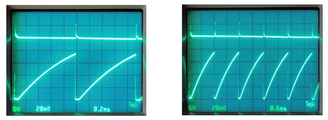
A ramp followed by a fast return shows that the circuit can charge a capacitance, fire and move on to the next cycle. The photograph compares time scales and signal shape; on its own it does not provide the current at the G1 terminal for each of the six anode currents of the Sylvania plate. This distinction makes it possible to recognize the result achieved by the 2016 model and to point to an additional, repeatable test.
When an application waveform is enough
In a relaxation oscillator the frequency can be dominated by the charging constant of the external capacitor and by the effective trip threshold. Reproducing the frequency is a relevant check for that topology. To isolate the tube parameters, on the other hand, one can vary bias, grid resistance and anode voltage separately, observing which quantities stay in agreement. Two models can produce the same period while differing in the load on the source or in the time the tube needs to regain control.
Tests that distinguish the different levels of model
Static curves
Compare grid current and the position of the zero at each anode current. For firing, repeat the anode sweep at several G2 values and with a declared grid resistance.
Waveforms
Measure turn-on, rise and recovery separately. For recovery, record how the threshold of the second pulse changes as a function of the interval between the two commands.
Bringing the 1957 RCA data into the SPICE comparison
The internal connection of G2 to K selects only one section of the problem. In the RCA tests even a zero-volt shield source feeds G2 through 1 kΩ. If the shield draws current, shorting it to K can produce a different potential. To compare the model with figure 3a this approximation must be made explicit. For figure 3b, acquired with the shield supply at +9 V, the three-terminal subcircuit lacks the necessary degree of freedom. A threshold difference between the panels is therefore also a test of the structure of the model.
A second comparison concerns memory. The internal node of an RC network can decay with an assigned constant even when the current the external circuit sees at G1 is almost zero. RCA’s figure 9 makes it possible to ask for both: how long recovery lasts and what current flows through the bias resistance while the tube recovers. Two simulations giving the same re-ignition instant can thus be told apart by the grid voltage and current along the transient. Olmstead and Roth, fig. 9.
Barnes and Wait’s three-gap model
In the 1993 model the discharge of the CX1171 crosses three gaps and the intermediate drift spaces. Figure 1 builds a progressively switching circuit element. A controlled source generates a voltage proportional to the product of the current through the branch and a control quantity that decays with time. Seen from the terminals, the branch thus has a variable effective resistance. The residual value can be chosen to obtain a given drop at a specified load current. The same choice then implies a drop proportional to the current in the branch.
Figure 3 shows a version in which the drift spaces are lumped with two of the discharge gaps. When a gap turns on, the redistribution of voltage drives displacement currents through the capacitances of the system. Figure 4 shows how the capacitance to ground affects the predicted cathode current. This sequence explains why a signal at the terminals can precede full conduction. In the Flash-Matic the corresponding question is how to distinguish a capacitive transient from the current that announces firing. The three-gap network belongs to the geometry of the CX1171. Barnes and Wait, 1993, figures 1–5.