

The 2D21 Thyratron: From Historical Curves to SPICE Models
8. How the return of control after the discharge is measured
Deionization as a circuit-dependent test
In 1949 Verzuh describes a method for deriving the recovery time with a calibrated time sweep. The experimental problem is to establish when, and under what conditions, the grid again prevents conduction. A test must define the end of the previous discharge, the voltages during the interval and the condition under which the anode returns positive. The residual current and re-ignition respond to this electrical history. The quantitative formulation must therefore identify the test to which each time belongs. Verzuh, MIT Research Laboratory of Electronics, Technical Report 101, 8 March 1949.
| Test | Quantity observed | Conditions to record |
|---|---|---|
| Return of control | First interval for which the tube stays off when the anode voltage is reapplied. | Current before extinction, grid resistance, bias and returning anode edge. |
| Re-ignition | Anode voltage at which the discharge restarts after a given interval. | Interval, shape of the applied voltage and state of the grids. |
| Afterglow | Current collected by an electrode after extinction. | Electrode observed, bias voltage, condition of the tube before extinction. |
| Repeated test | Distribution of times or fraction of re-ignitions. | Sequence of cycles, classification criterion and number of repetitions. |
In Romanowitz’s 1947 bulletin the title explicitly identifies measurements, analysis and the statistical nature of deionization time in a mercury-vapour tube. The 1950 work with Dow continues on the statistical character and the physical mechanisms. The 1950 paper documents geometry, circuit and the counting of re-ignitions on the KU-627. The 1947 bulletin has yet to be compared with this later publication. Romanowitz and Dow, Transactions AIEE, 1950.
Malter and Boyd refer to Studies of Thyratron Behavior by Malter and Johnson in their discussion of the residual plasma, the ion sheath and the restoration of control after the discharge is interrupted. The two works make it possible to follow the step from the study of the afterglow to the proposal of entrusting firing and recovery to two distinct electrodes. Malter and Johnson, RCA Review 11, p. 165 ff., 1950.
The re-ignition probability of the KU-627
In 1950 Romanowitz and Dow use a Westinghouse KU-627 mercury-vapour tube. Figure 1 shows its dimensioned geometry. The circuit of figure 2 takes the anode to a negative potential to extinguish the discharge and then reapplies a positive voltage after an adjustable interval. If the tube restarts, the anode voltage drops back towards the conduction level. Figure 3 defines the expected swings and figure 4 makes it possible to recognize them on the oscillograph, including the case of a rare re-ignition.
The authors vary the interval and count how many tests end with a new discharge. Among the intermediate points they usually look for 5%, 50% and 95% re-ignitions. To fix the operating limit they lengthen the interval until they observe fifty consecutive tests without re-ignition. The experimental result is therefore a frequency observed on a finite sample. The position of the median and the time obtained with the fifty-test criterion answer two different questions.
Figures 5 and 6 reorganize the same data, highlighting respectively the grid-circuit voltage and the anode current before extinction. Among the other documented conditions are the resistance of the grid network, the negative anode voltage during the pause, the positive voltage reapplied and the temperature of the condensed mercury. The last is specific to the tube used. For the 2D21 the statistical method can be taken up, specifying in the model which re-ignition probability the stated time represents. Romanowitz and Dow, figures 1–8.
Malter and Boyd: assigning firing and recovery to different electrodes
Malter and Boyd distinguish grid emission, which can shift the control characteristic, from the collection of positive ions during the afterglow, which can delay its recovery. A smaller grid resistor reduces the conversion of both currents into voltage changes, at the cost of lower sensitivity to a current signal. In their experimental structure a thin electrode receives the firing command, while a second electrode biased at low impedance favors recovery. The experiment documents two distinct functions of the grid and a trade-off between sensitivity and recovery. The naming of these two electrodes must be kept distinct from G1 and G2 in the 2D21. Malter and Boyd, Proceedings of the IRE 39, pp. 636–643, 1951.
In Malter and Boyd’s comparison, the tube conducts for 6 µs at 250 mA. After the interruption, a 200 V test anode pulse checks the return of control. In figure 11, when the two grids of the prototype are at the same potential, the behavior approaches that of the conventional tube. In figure 12 the series resistance makes visible the advantage of the small-area control electrode. The coupling capacitance also contributes to the response. Table I gives 0.83 pF between trigger grid and anode in the prototype, against a nominal value of 6 pF between grid and anode in the conventional tube. The first figure comes from a bridge measurement on the experimental model. The second is the catalog term of comparison.
To distinguish thermionic emission from the grid from ion collection, the authors fit thermocouples to the grid and anode. In the emission test they keep the grid at −25 V with respect to cathode and anode during the reading. Figure 5 follows the heating of the electrodes and figure 6 shows how the emitted current evolves. The result gives an experimental meaning to the thermal history of the grid. Two readings at the same bias can correspond to different temperatures and surface conditions. Malter and Boyd, Proceedings of the IRE 39, 636–643, figures 5–6 and 10–12.
Reich derives the grid voltage from load lines
In 1957 Herbert T. Reich publishes a one-page note that can be read as a two-step graphical construction. At the time of interruption of the anode current and at four later, equally spaced instants, he draws five grid current–voltage characteristics. He assumes that, at fixed grid voltage, the positive ion current decays exponentially with the plasma density. For each bias network he then draws the load line. The point at which it cuts each characteristic gives a current–voltage pair at the same instant.
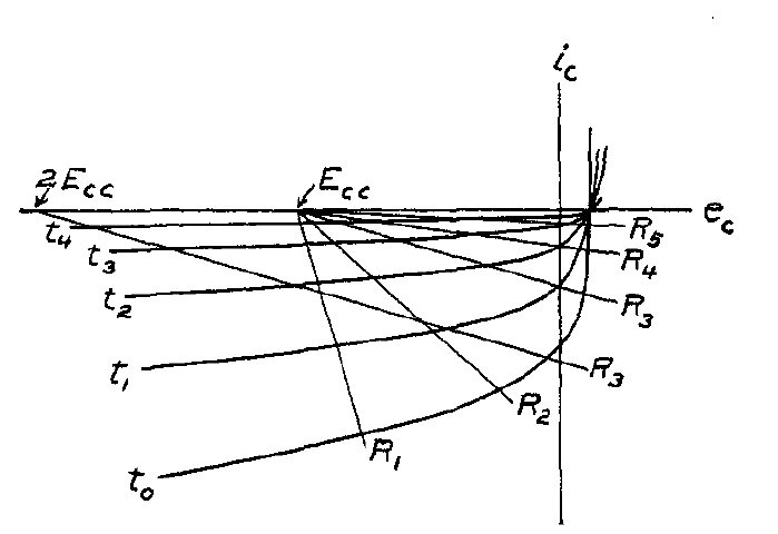
In figure 2 Reich plots against time the voltages read at the intersections. With a high resistance the line meets, for several instants, the region beyond the knee, where the characteristics are close together. The grid voltage can thus stay small in magnitude while the plasma decays. Reducing the resistance, or increasing the magnitude of the bias, the grid reaches a given fraction of the supply voltage sooner. The two figures represent a graphical calculation compared qualitatively with the experiments of Malter and Johnson. For a 2D21 model, this reading indicates which variables to plot together after extinction: grid current, actual voltage on the pin and voltage of the bias source. H. T. Reich, Thyratron Grid-Control Recovery, 1957, p. 287.
The diffusive model and its relation to an RC circuit
In Hill’s thesis the residual density can decay with several time scales. For a diffusive mode, \(\tau=\Lambda^2/D_a\), where \(\Lambda\) is the effective diffusion length and \(D_a\) the ambipolar diffusion coefficient. Two regions can give a term of the form \(A e^{-t/\tau_1}+B e^{-t/\tau_2}\). If the same diffusion coefficient applies, halving the characteristic length reduces the mode time to a quarter. Real values depend on gas, geometry, initial conditions and the limits of the diffusion model. Hill, Texas Tech University, 1978.
An RC network can reproduce one or more exponentials with effective constants. To give it quantitative meaning one must specify how the equivalent internal voltage is reflected in the grid current or in the observed re-ignition potential. The comparison between simulation and test must therefore include the threshold condition as well as the shape of the decay.
The oscillograms of Malter and Johnson
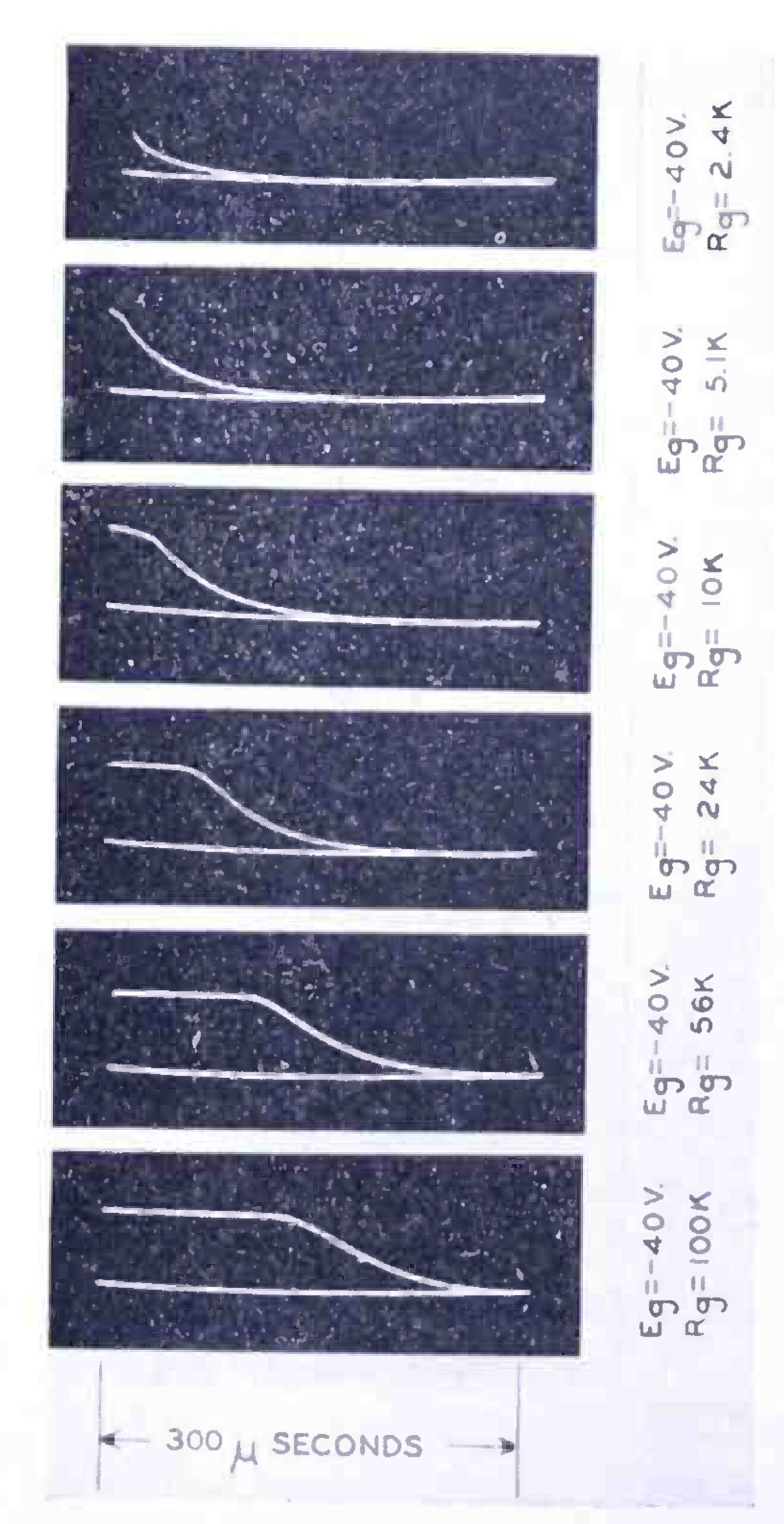
In the first part of the 1950 RCA study the commercial tube contains argon and mercury vapour. In figure 3 the source bias is fixed at −40 V. After the anode current ceases, the grid potential can stay close to that of the cathode for part of the trace. Increasing the resistance lengthens this interval. The authors reconstruct the current from the voltage across the resistance and in figure 6 find a decay with a time constant of about 52 µs for the test described. The legend under the traces gives the time base and makes it possible to distinguish the almost horizontal segment from the return towards the bias. Malter and Johnson, part I, pp. 170–171.
Their interpretation provides a discriminating test. If the residual ions sustain a voltage drop close to the available bias, the grid stays near the cathode potential and can also collect electrons. When the ion flux decreases enough, the voltage returns towards that of the source. A slower functional recovery can therefore be observed even with a practically unchanged rate of ion loss. A model that automatically made the diffusion time constant grow with resistance would confuse the two causes.
The second part, signed in the order E. O. Johnson and L. Malter, looks for the limit of this explanation. By applying a sudden change of bias shortly before the re-ignition test, the authors also observe an effect of the grid’s time history. They discuss the time required for the charge distribution to regain a quasi-equilibrium condition. In one of the tests they expressly identify a 2050: the measurement offers a physical and metrological comparison, but its numerical value does not automatically characterize the xenon 2D21. Johnson and Malter, part II, pp. 178–189.