

The 2D21 Thyratron: From Historical Curves to SPICE Models
9. The 2D21 measured with pulses by Olmstead and Roth
In June 1957 John A. Olmstead and Melvin Roth, of the RCA tube division at Harrison, published thirteen pages devoted entirely to the 2D21. Part of the research came from Olmstead’s thesis work at the Newark College of Engineering. Their article makes it possible to connect two tests that a data sheet compresses into a few lines: the minimum duration of the excitation needed to cause firing and the ability of the grid to block a second application of anode voltage. Pulse-Firing Time and Recovery Time of the 2D21 Thyratron, RCA Review XVIII, pp. 272–284.
Which event marks firing?
The bench of figure 1 applies a square wave to the anode and a delayed positive pulse to the grid that falls during the high anode level. The oscilloscope shows whether the anode stays at the applied voltage or whether the voltage collapses because of conduction. Shortening the pulse, one meets a critical duration: beyond that point, its final part can be suppressed and the discharge develops anyway. The instant at which G1 loses control in principle precedes the completion of ionization. The authors judge the difference negligible on the 2D21 in their tests. This definition allows a comparison with a simulation even when the simulator describes the discharge through an internal variable invisible on the bench.
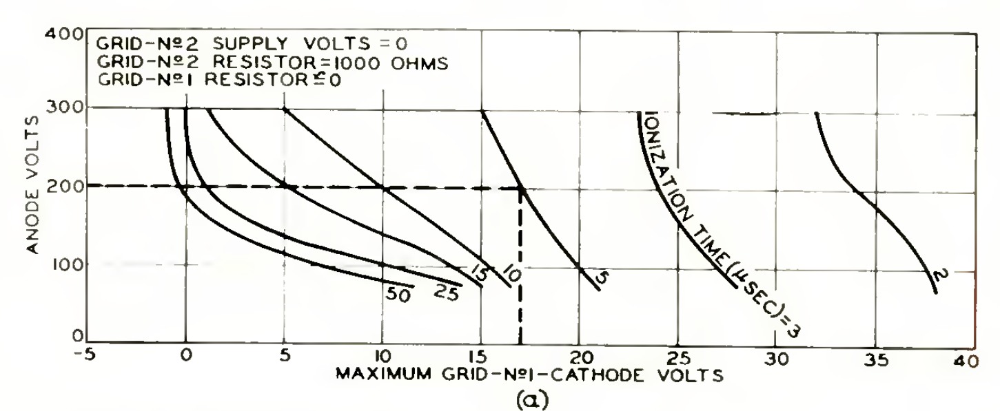
Figure 3a presents a constant-time family. At 200 V on the anode, with the G2 supply at zero, RCA reads an effective +17 V between G1 and K to fire within 5 µs. In figure 5a, which instead gives the minimum limit, a pulse of the same duration can already produce firing above +8 V. The 9 V between the two readings is not the hysteresis of a single specimen. It is the gap between two published criteria, “may fire” and “voltage required within the prescribed time”. For a coincidence circuit the first limit matters even when the aim is to avoid an accidental command. RCA, figure 5, p. 277.
The pulse at the generator and the voltage actually applied
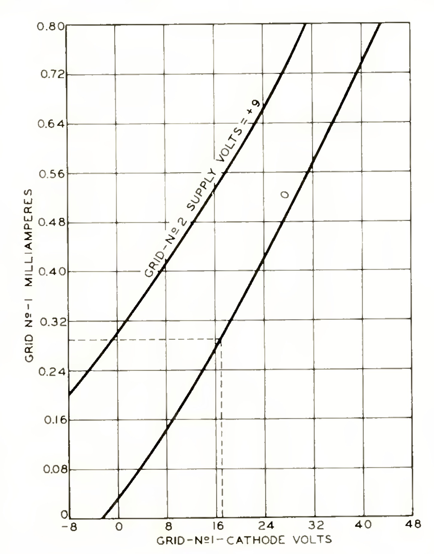
In the RCA example figure 4 gives about 0.29 mA before firing at +17 V on G1. This is a transient positive excitation condition. The nanoampere current of the static Sylvania plate belongs to another region of the characteristic. A practical distinction follows for the historian of models: a branch able to reproduce the photocell load near cut-off could underestimate by several orders of magnitude the load of a positive pulse source. A meaningful comparison requires sign, voltage, duration and state of the tube.
An arithmetic check shows the size of the correction. With 46.5 kΩ in series, 0.29 mA produces a drop of about 13.5 V. In the paper’s example the resting point is −75 V. A source swing of about 75 + 17 + 13.5 = 105.5 V is therefore needed, rounded by RCA to 106 V. The value useful for reading figure 3 remains +17 V. Entering 106 V on the grid axis would change the meaning of the measurement. The authors’ numerical example, p. 283.
The test pulse after extinction
For recovery, figure 6 uses a different sequence. First a repeatable conduction is established. After the end of the current a preset interval is waited out and a test anode pulse is reapplied. For the same interval, test voltage and previous current, the bias that just prevents the second discharge is sought. The grid may have recovered enough control to pass this test even if charge carriers still exist inside the tube.
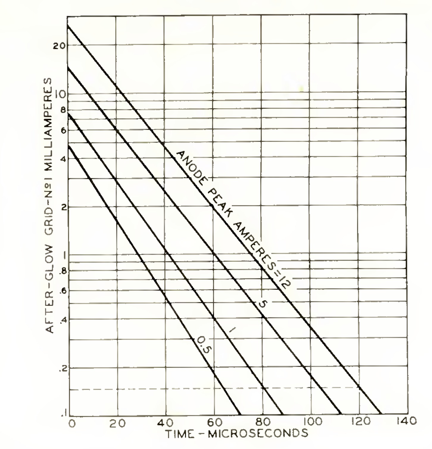
For a reapplication of 200 V after 120 µs, the text compares about −68 V on the grid after a 12 A anode pulse with about −38 V after a 5 A one. These are peak currents of the historical tests. Figure 9 separately gives the residual current that alters the bias through the external impedance. This is why the same interval can be enough in one test and insufficient in the other. Recovery measurement and comparison of figures 7 and 8, pp. 279–281.
A test for later models
| Comparison | Observable to compare with the simulation |
|---|---|
| Figures 3 and 5 | At finite duration, minimum and maximum voltage envelopes as a function of anode and shield. |
| Figure 4 | G1 current during the positive swing, before the tube conducts. |
| Figures 7 and 8 | Critical voltage to avoid a second discharge after a defined interval. |
| Figure 9 | Residual current as a function of time, distinct from the binary re-ignition criterion. |
These data make it possible to check separately a model of firing and one of the memory of the discharge. An ideal switch with constant delay can imitate a single outcome, but leaves undetermined how much the required voltage should change when the pulse is shortened. An exponential internal decay can reproduce a residual curve: to predict re-ignition it must also generate the correct terminal current and respond to the test voltage. The RCA work thus narrows the ground for any claim of novelty. Extensive dynamic measurements on the 2D21 already exist; how well a compact model reproduces them together with the GE static characteristics remains a distinct question.
In 1959 Adati and Sawa take up Olmstead and Roth’s comparison on the 2D21. By changing the interval between two commands they observe that the previous discharge can still shift the firing threshold after the tube has regained the ability to block the anode voltage. Page 17 follows figures 4–7 and the move to triggering through a ferrite core. Adati and Sawa, article and PDF.