

The 2D21 Thyratron: From Historical Curves to SPICE Models
12. From historical precedent to a quantitative model of the 2D21
What has already been developed on Giux-Lab
The Level-1 grid-current model uses the GE curves during conduction. It normalizes the grid current by Ia, refers the voltage to V0 and uses two scales for the branches of opposite sign. One structure reconstructs the characteristics when the parameters of the family are known. The positive law is a normalized exponential, the negative one a combination of exponentials constrained to characteristic points. Both pass through the zero of the current. The published version makes available the consensus curves, the parameters and the uncertainty material from replicated digitizations.
The parametrization of V0 as a function of Ia turns out to be smoother than that of S− in the reported checks. To support a predictive surface over the continuous range of Ia it must be shown that the parameters can also be reconstructed for families left out of the fit. The 5 mA family must be kept explicit as a possible distinct regime. At 300 mA the limits of the trace reduce the identifiability of some parameters.
How to measure the agreement
On a family observed at \(I_a=I_{a,k}\) one can define the vertical residual \[ r_{ik}=I_{g1,ik}^{\mathrm{digit}}-\widehat{I}_{g1}(V_{g1,ik},I_{a,k}). \] It must be examined as a function of voltage and separately for each anode current: a root-mean-square value alone can hide a systematic deviation in the transition zone or on the plateau. If the uncertainty on the voltage is significant, the local slope can turn a small horizontal error into an apparent current error. In the steep segment an assessment is therefore needed that takes account of both axes and of the correlation introduced by the calibration.
Leave-one-family-out validation measures interpolation within the same source. A data sheet from another manufacturer is a distinct check, provided the test circuits are compared. A measurement on physical tubes finally adds information on the variability between specimens. Documenting which test was carried out makes the scope of a quantitative model verifiable.
How large is the error on the GE curves?
For the negative branch of the Level-1 model, the Giux-Lab work publishes both the root-mean-square deviation in units of current and the deviation relative to the local spread of the digitizations. Reading the two numbers together changes the ranking of the most difficult families. In the table the absolute deviation is converted to microamperes to make the comparison more immediate. Level-1 analysis, “Quantitative verification” section.
| Anode current | RMSE on the negative branch | RMS of the normalized residual |
|---|---|---|
| 25 mA | 6.4 µA | 0.53 |
| 50 mA | 10.8 µA | 0.93 |
| 100 mA | 23.9 µA | 1.98 |
| 150 mA | 26.0 µA | 1.83 |
| 200 mA | 15.7 µA | 0.86 |
| 300 mA | 104.9 µA | 1.24 |
At 300 mA the absolute deviation is the largest, but so is the spread of the trace. At 100 mA the discrepancy weighs more relative to the estimated uncertainty. The roughly 300 samples of each curve are interpolation points. Going down to about 30 points, between 25 and 200 mA the change in QA stays below 0.2% and that of U20 below 0.3%. This check concerns the numerical density of the representation. A second series of tubes or another documentary source would verify a different property.
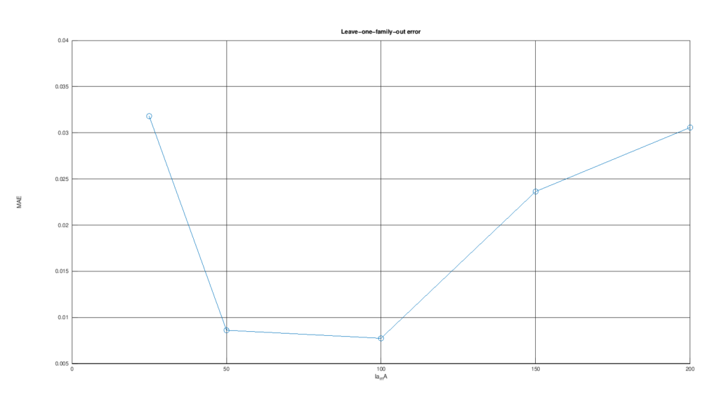
Comparing the equations of the models
Before the comparison, voltages, currents and parameters are brought to the same convention. One then checks whether the laws become equivalent through translations, normalization or change of variables. Exponents, separability, thresholds, limits and asymptotes must be examined, together with slopes and curvature. For a multivariable surface, the mixed derivatives of the Hessian matrix can reveal a coupling between the variables even when some sections appear to coincide.
Any common curve after normalization must be checked on several families and in their respective measured ranges. The parameters must be compared one by one, keeping physical, empirical and numerical parameters distinct and checking correlations and identifiability. Errors by family, residuals, parameter covariance or confidence intervals, where they can be estimated, and verification on data held out of the fit make it possible to grade the comparison between equivalence, the same limiting law, quantitative extension and different mathematical structure.
The outcome of the survey
The literature contains experimental curves, local laws, quantitative studies of firing and recovery and a functional macromodel that declares compatibility with the 2D21. In the sources examined, the search remains open for an integrated parametrization of the 2D21 that identifies, documents and quantitatively verifies several of the manufacturer’s families. For the Flash-Matic receiver the operational question is how much threshold and command margin change when G2, the impedance of the grid network and the recovery of the discharge are represented.