

Manual Digitizing: Adding, Selecting, Moving and Deleting Points
This guide shows how to turn clicks on the image into calibrated numerical points with Curve Digitalizer, select a curve, correct coordinates with Move and delete individual points with Delete. The example uses a Session with a synthetic graph and makes it possible to tell the image pixels apart from the stored scientific points.
1. Source Image and Scientific Data Are Two Different Objects
The example uses a synthetic 1280 × 900 pixel PNG with five colored traces. To illustrate the manual operations, only the blue line and the green line are digitized.
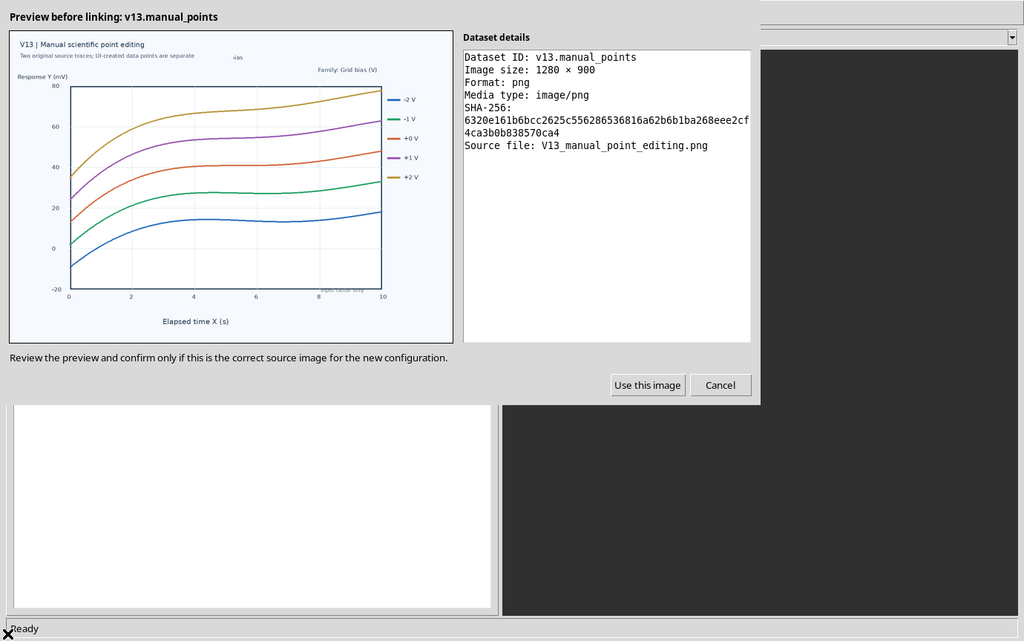
The five lines and the legend belong to the raster pixels. At the start, none of them is a scientific Series object: to create the numerical curves you need to use the Curves tab. The source is registered as a canonical Image Dataset with the image.raster contract; it is not a laboratory experiment.
2. Axes and Calibration Are Needed Before Adding Points
The configuration uses Elapsed time on the X axis from 0 to 10 s and Detector response on the Y axis from −20 to 80 mV, both with a linear scale. The Set BL, Set BR, Set TL and Set TR buttons were used to acquire the four real corners of the graph.
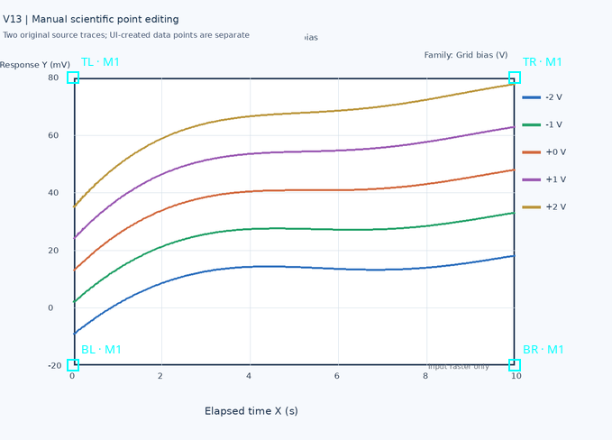
Once complete, the calibration was classified accepted with the Accept control of Calibration measurements. The two curves to be digitized share the same perspective transformation; no separate axes or homographies were invented.
3. The Point interaction Group of the Curves Tab
In the Curves tab, below the list of series, there is Point interaction, which offers six modes: Add, Move, Delete, Add guide, Edit proposal and Add correction point.
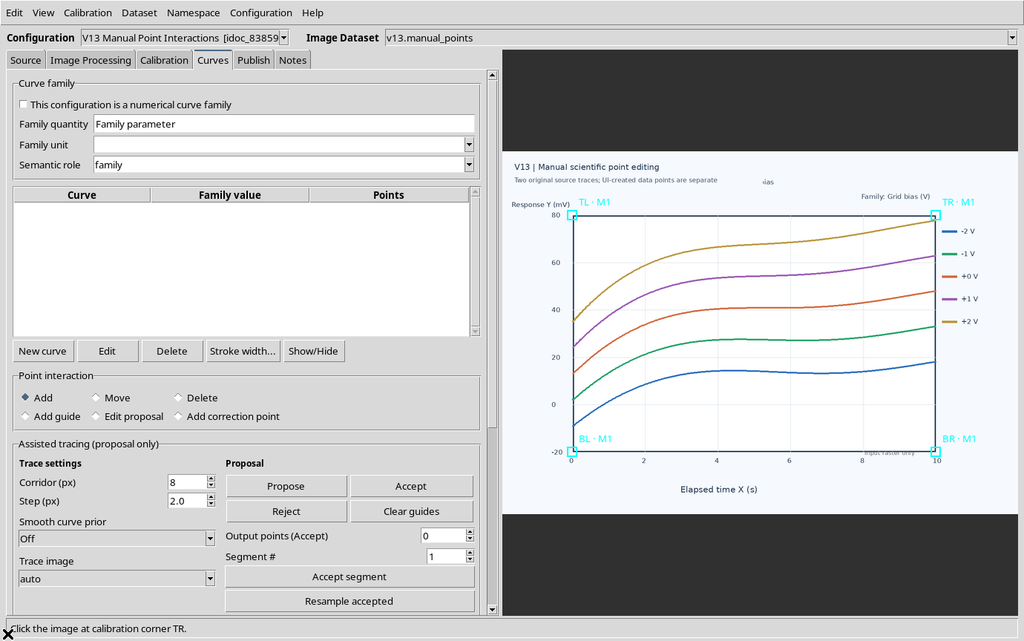

Manual digitization uses Add, Move and Delete. Add guide, Edit proposal and Add correction point concern assisted tracing, described separately.
4. Creating Two Curves with New curve
From the Curves tab, the objects Blue manual curve and Green manual curve were created with New curve, leaving This configuration is a numerical curve family disabled.
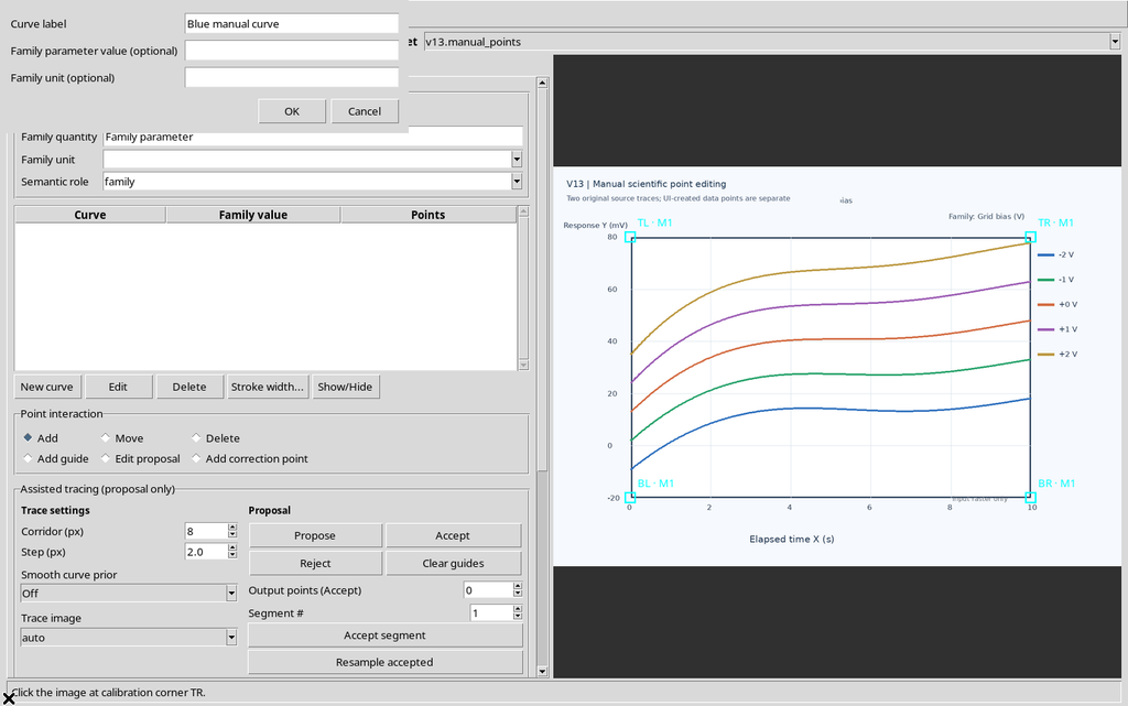
The table showed two rows with Points = 0, even though the two lines were already present in the PNG.
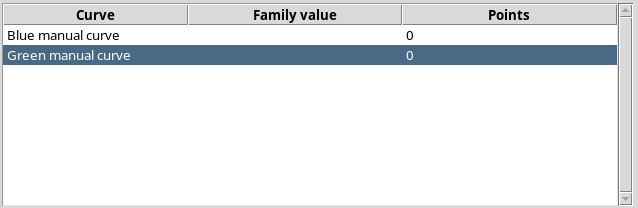
Each curve has a stable identifier distinct from the displayed label. The two series were created separately and with zero numerical records, not as a parameterized family.
5. Add Without an Active Curve: Correct Refusal
The Add mode was selected and the image clicked before a curve was created or selected. The Viewer showed the message:
Create or select an active curve first.
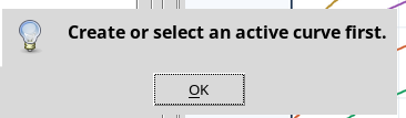
No point, new curve or Dataset was created. Add cannot guess which series a click should belong to.
6. Selecting the Blue Curve and Disabling Snap to dark
With Blue manual curve selected, the Add mode was set and Snap to dark kept disabled.
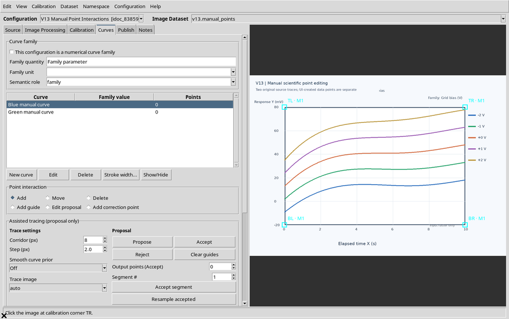
With snapping off, Manual click and Stored pixel are identical to each other in the record for every insertion.
Active snapping and its options are covered in a later chapter.
7. First Point: Chosen Pixel and Calibrated Coordinates
The first click on the blue trace created a manual point with an overlay on the graph.
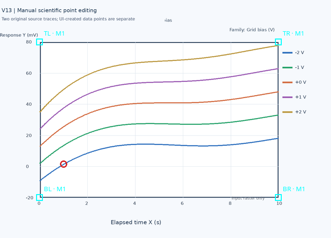
The frame below the interaction modes showed:

| Field | Interface result |
|---|---|
| Manual click X/Y | 263.367 / 618.518 px |
| Stored pixel X/Y | 263.367 / 618.518 px |
| Scientific X | 1.000 s |
| Scientific Y | 1.630094 mV |
The record also contains its own ID, the manual origin and the coordinates in pixels and scientific units. The physical value comes from the four calibrated corners, not directly from the color of the PNG.
8. Five Actual Points on the First Curve
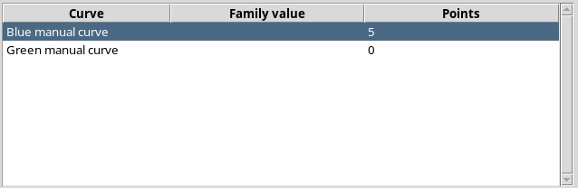
Four more points were added along the blue trace, at increasing X. The table showed Blue manual curve — Points 5; the points are stored in the Workspace managed by the CORE, so they do not exist only in the interface.
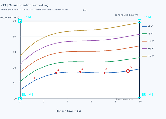
The five points have distinct UUIDs, a stored source position and calibrated X/Y values. They are not automatic proposals and not rows of an already published Dataset.
9. Show point numbers Changes Only the Presentation
Enabling Show point numbers, the Viewer drew the labels 1–5 next to the points of the curve.
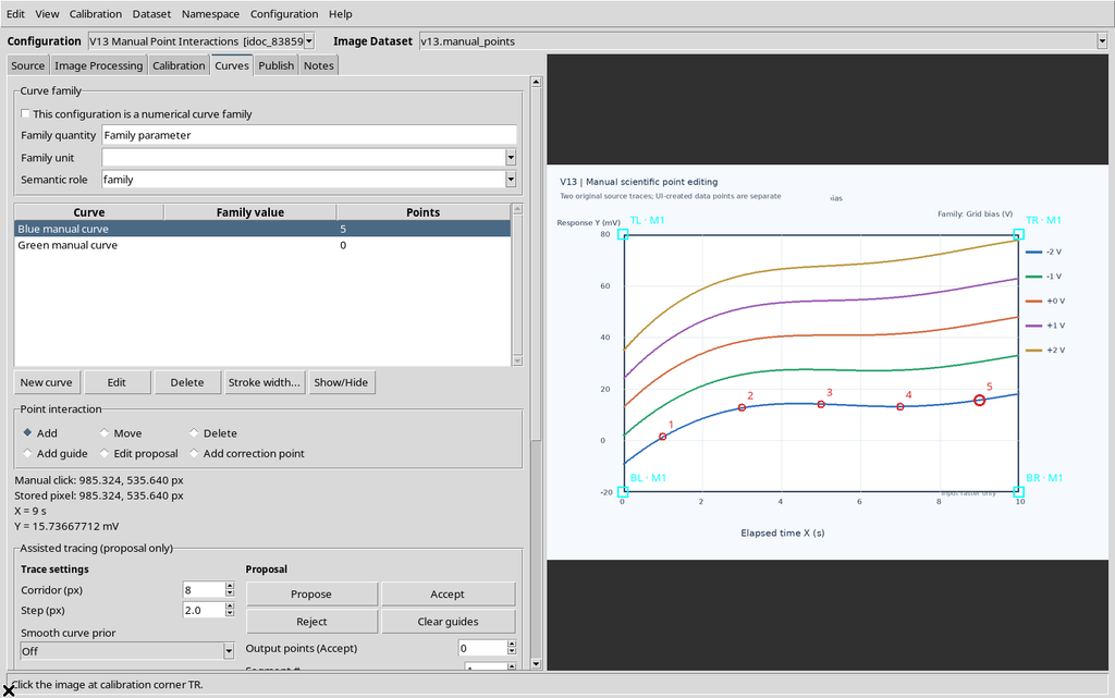
Enabling it did not alter the five scientific records. The visual number must not be treated as a persistent ID: the displayed sequence can change with the ordering criterion and after points are removed or re-inserted.
10. Selecting the Green Curve Without Losing the Blue One
With a click on the Green manual curve row, the five blue points already acquired stayed in place.
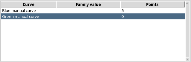
The active row identifies the series that will receive the next Add clicks and in which points will be looked for when selecting and editing. Changing the active series does not transfer points from one curve to another.
11. Adding Five Points to the Green Curve
Five real clicks created as many points on the green trace, for a total of ten points, five blue and five green.
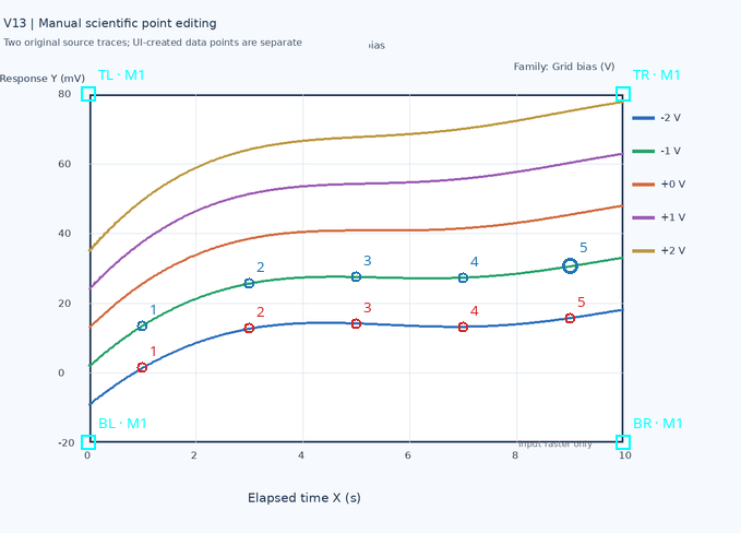
The IDs are all different and the framework keeps the manual coordinates, the stored pixels and the calibrated values.
12. Move Selects the Point in the Active Curve
After choosing Move, the third green point was clicked directly on the canvas. The selected marker appeared larger.
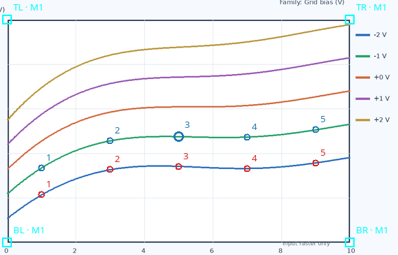
The GUI showed its data in the detail section:

Selection alone does not change the coordinates.
13. Real Dragging and X/Y Recalculation
The selected green point was dragged with real Tk press, motion and release events on the ImageCanvas.
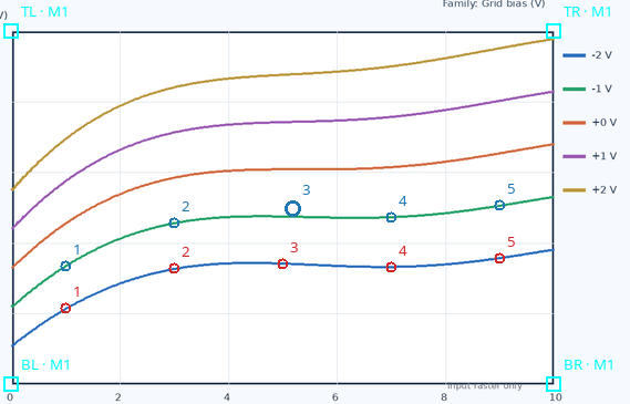
The point frame reported the new coordinates:

| Property | Before | After |
|---|---|---|
| Pixel X | 624.345 | 640.921 |
| Pixel Y | 465.655 | 452.763 |
| Scientific X | 5.000 s | 5.184 s |
| Scientific Y | 27.649 mV | 29.843 mV |
Dragging modifies the point, it does not create a new one.
14. A Second Move to Correct the Position
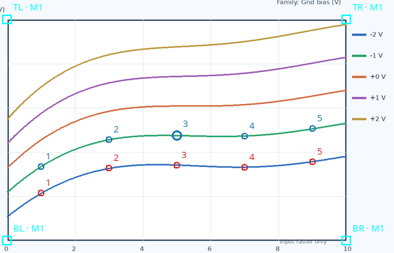
With a second drag the same point was brought back close to the original green trace.
15. Clicking an Empty Area Clears the Selection
A click in an area of the raster with no points removes the highlight of the selected point in Move mode.
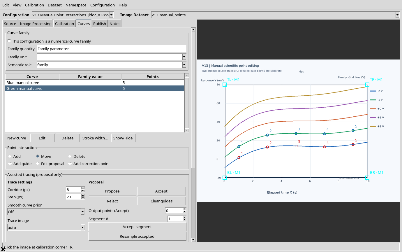
16. Only Points of the Active Curve Can Be Selected
With the green curve still active, clicking the marker of a blue point did not select it. After selecting the blue curve in the table, the same point became selectable with Move.

Point selection is limited to the active curve. Before moving or deleting a point close to several lines, check which Series is selected. The figure shows the selection available for a point of the active curve.
17. Delete as a Direct-Click Mode
The Delete mode of the Point interaction group works on scientific points, not on whole curves. A click in an empty area removed nothing.
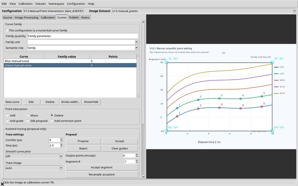
Clicking a point of the green curve instead, the count went from 5 to 4 and the corresponding UUID disappeared.
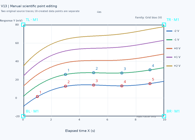
All five blue points stayed unchanged. The Delete button below the Curves table has a different meaning: it concerns the whole selected curve.
18. Deleting from the Keyboard with Delete
To show the second path, the Move mode was chosen, another green point was selected and then the Delete key was pressed.

The green count went from 4 to 3, without changing the blue curve.
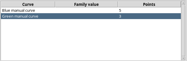
The selection was cleared after the deletion. Pressing the key did not delete the whole series.
19. Edit → Delete selected point in the Menu
A blue point was selected and the Edit → Delete selected point command of the native menu was used.
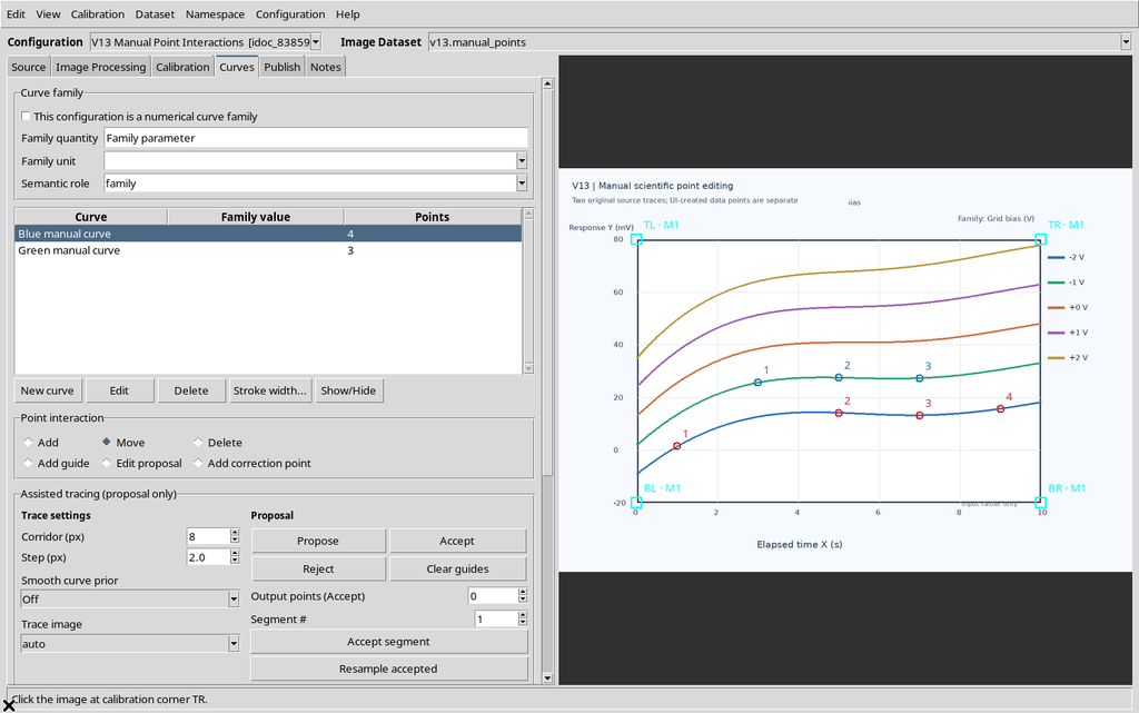
The selected point was deleted and the blue count went temporarily from five to four. The three green points stayed identical. Do not confuse Delete selected point with Delete selected curve….
20. Re-inserting the Same Pixel Generates a New ID
The blue point just deleted was added again with Add, clicking the same position on the canvas.
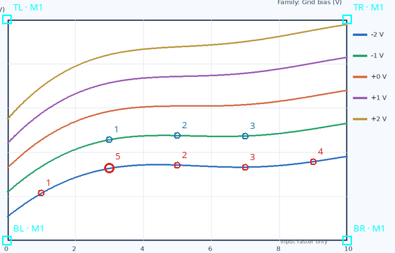
The new record has the same coordinates as the previous one but a different UUID: the old, deleted identifier is not recycled. Editing with Move keeps the identity; deletion followed by insertion creates a new scientific object.
21. Numbering and Insertion Order
In the observed case, insertion order was in use. The point recreated near X=3 s became the fifth point of the curve, not the second.
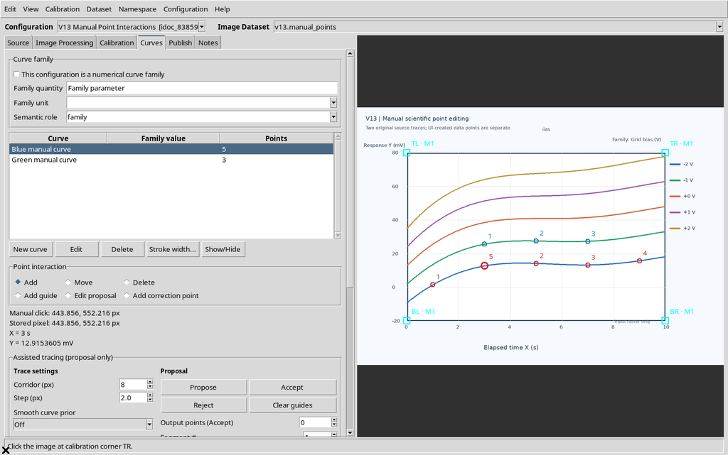
The displayed number follows the order of the points in the curve, but it is not an immutable key. Ordering modes, monotonicity constraints and Undo/Redo are covered in the dedicated section of the guide.
22. Hiding a Populated Curve Does Not Delete the Pixels
With five blue points still present, Show/Hide was used on the blue curve.
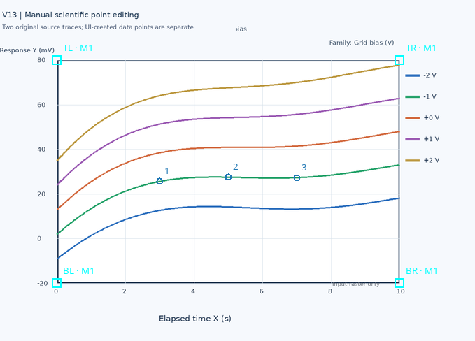
The blue numbered markers disappeared, but the blue line drawn in the PNG stayed visible. The CORE confirms that the same five blue points and three green points were still present: only the visibility field changed.
23. Restoring the Markers Without Regenerating the Points
With a second Show/Hide, the blue curve became visible again.
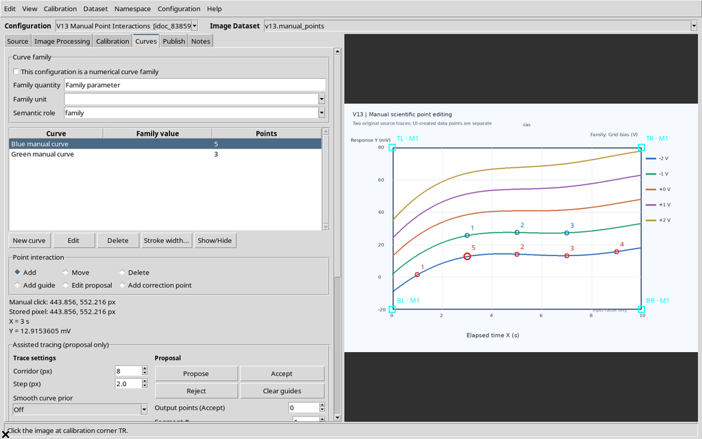
The number of points, the physical coordinates, the IDs and the SHA-256 of the source image stayed identical. No new acquisition and no copy of scientific data took place.
24. Hiding Only the Numbers
Turning off Show point numbers, only the numeric labels disappeared, not the markers.
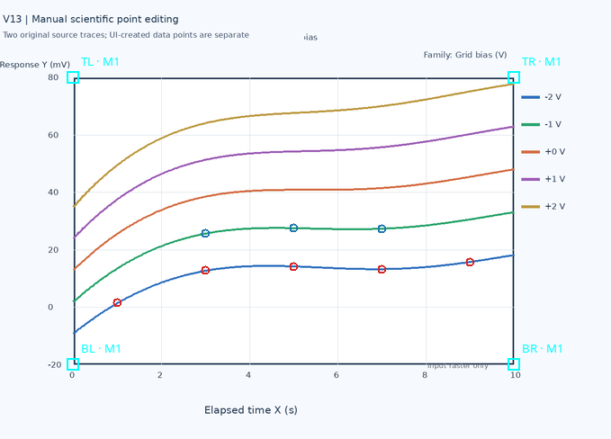
The numbering was then re-enabled and saved. Show/Hide changes the visibility of the curve; Show point numbers changes the presentation text associated with the points.
25. Scientific Points Cannot Be Added from the Calibration Tab
With Add active, the Calibration tab was selected and the image clicked.
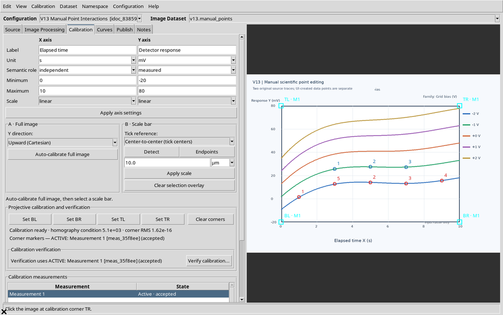
The Viewer added no points: the check on the scientific data still returned five blue points and three green points. The manual digitization modes belong exclusively to the Curves tab.
26. Saving, Closing and Reopening the Same Session
The configuration was saved with Configuration → Save configuration, closed normally and reopened with Viewers → Digitalizer in the same synthetic Session.
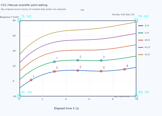
The Workspace kept all eight final UUIDs, the manual and scientific coordinates, the two curves, the accepted calibration and the SHA-256 identity of the source. The temporary point selection was not kept as scientific data. The Show point numbers presentation option stayed enabled.
27. Essential Operating Procedure
To repeat the operation: choose the source, set four valid corners, create and select a curve, click Add on the real points; use Move to select and drag, or Delete for a direct click. The Delete key and Edit → Delete selected point, instead, act on the previously selected point. Save and check that the configuration reopens correctly.