

Canvas: Zoom, Pan, Display and Overlays
In this chapter (V05), visual pixel transformations are distinguished from calibration, scientific data and publishing.
1. Purpose, Requirements and Test Source
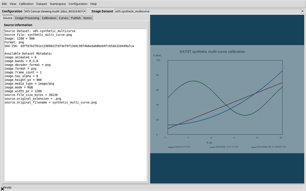
The Curve Digitalizer canvas lets you examine a raster figure precisely, zoom into areas, move the view and adjust appearance and markers. Viewing is not a digitization already performed: the three colored traces in our figure are initially just pixels of the source image.
To reproduce this work you need an open GX-TXT Session, a Digitizer Configuration and a compatible canonical Image Dataset, linked through Use this image. The Session of guide V05 contains a single image.raster Dataset, named v05.synthetic_multicurve in the example, a 1280 × 900 pixel PNG. Its SHA-256 is:
ddffb7b3761e12989022fdf4e79f13ddc99f4b6eda68beb97c65de32d449a7ca
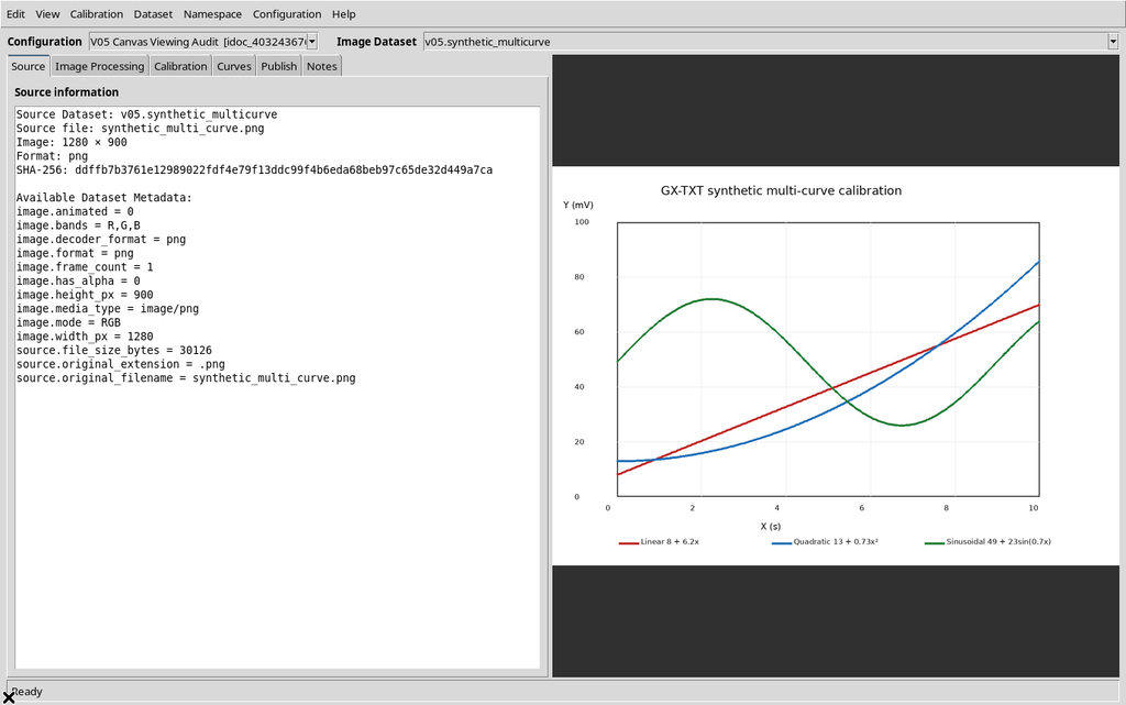
2. Scale and Coordinates: The Canvas Is Not the Original Image
Rendering keeps the original pixels and the canvas coordinates distinct. The presentation relationship is:
canvas_x = offset_x + scale × pixel_xcanvas_y = offset_y + scale × pixel_y
The inverse transformation is pixel_x = (canvas_x - offset_x) / scale, and likewise for Y. scale indicates how many canvas pixels represent one pixel of the figure, not the physical factor of an X/Y calibration.
The status bar and the scientific tools work on the coordinates of the original pixels, not on the coordinates altered by zoom and pan. The values are those verified in the isolated copy; they change if the image or the window size changes.
3. Mouse-Wheel Zoom: Button-4 and MouseWheel
To zoom into an area of the raster, place the pointer over the image and roll the wheel upward. On Linux/X11 the widget intercepts Button-4 to zoom in and Button-5 to zoom out; it also handles the MouseWheel event with a positive or negative delta.
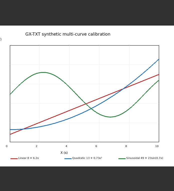
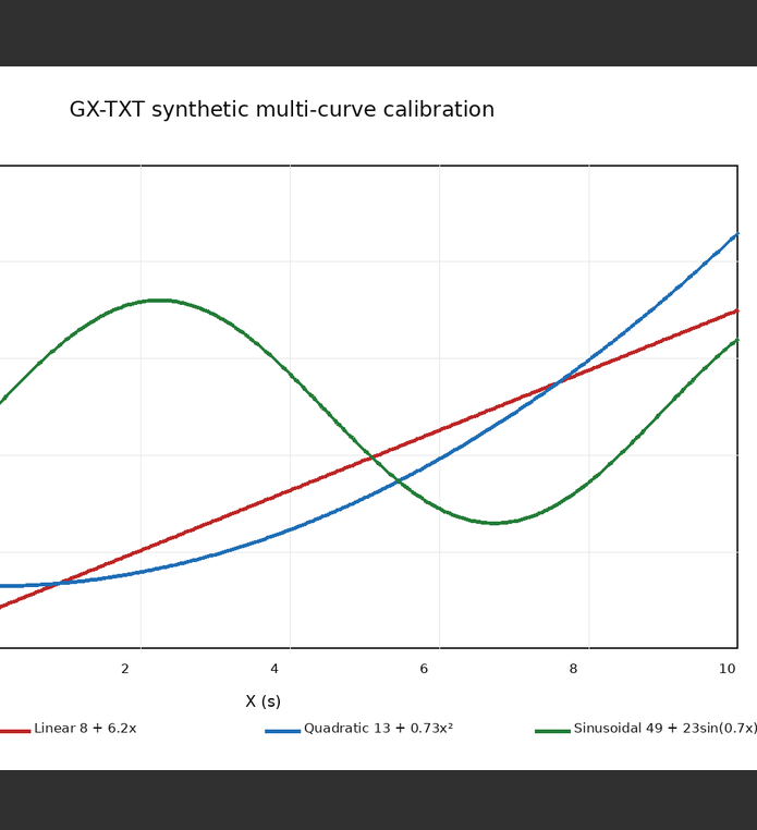
Zooming takes place around the pointer position.
4. Pan: Dragging with the Middle Button
With the middle button held down, drag the canvas in the desired direction. The image is shifted visually; the scale stays at its current value. On a mouse with a clickable wheel, the wheel acts as the middle button.
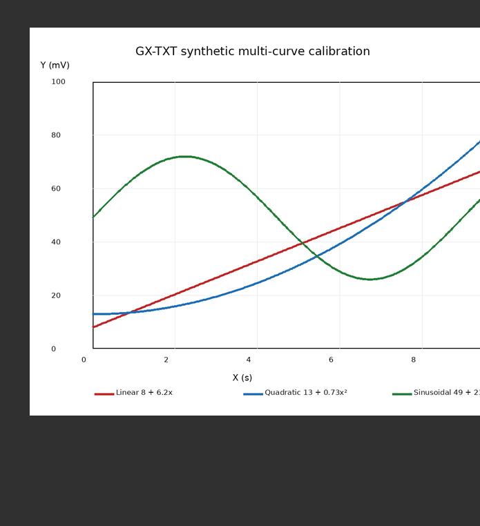
Panning does not perform a calibration, does not correct the position of the source points and does not update the numerical values of a curve. It only changes the visible portion of the raster.
5. Right-Button Pan and How It Differs from Context Menus
Dragging with the right button is also available. In the Source tab the image was moved by −48 pixels in X and +84 pixels in Y, without changing the scale or the content of the Dataset.
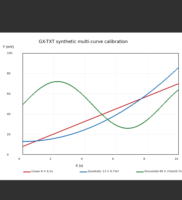
The interface, however, makes a distinction: in the Curves tab, a right-click on a guide, a proposal point or a scientific point can open a context menu instead of starting a pan. The behavior on scientific points will be described in later chapters.
If you simply want to navigate an area containing many markers, the middle button avoids the ambiguity of the context menus.
6. View → Fit image to window
When the graph is zoomed in or panned out of the viewport, select View → Fit image to window. The command recalculates the scale so that the complete raster fits in the canvas, and centers it in the unoccupied space.
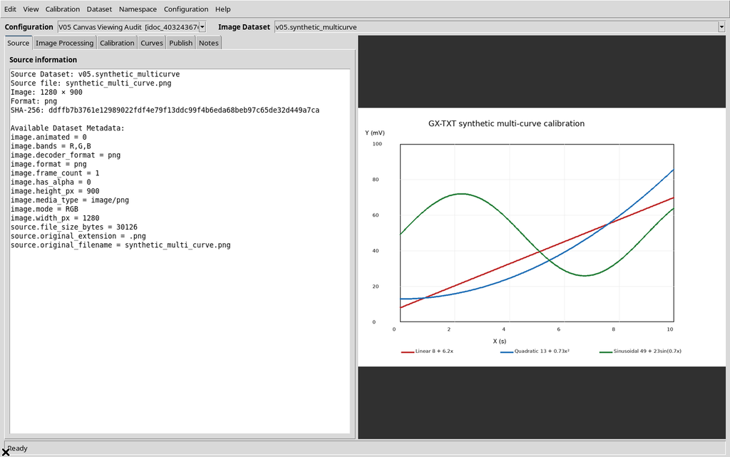
The rule is scale = min(canvas_width / image_width, canvas_height / image_height), limited to the values allowed by the widget. Fit does not return to a fixed 100% magnification: it computes the fit to the available size.
7. Status Bar and Cursor Coordinates
When the cursor is moved over a point that actually belongs to the image, the bottom bar reports Pixel X,Y and the current mode.
At canvas coordinate (235, 266) with the fitted view, the Viewer shows Pixel X,Y: 432.806, 237.281. These values match the inversion of the zoom/pan transformation given above, within rounding to three decimal places.

Moving the cursor outside the image, the bar went back to Mode: add without raster coordinates. Once a calibration is available, the bar can add the scientific X/Y coordinates (and Y2, if present).
8. Zoom Limits and View Recovery
Scale limits are enforced, preventing repeated wheel events from producing numerically uncontrolled transformations:
| Limit | Value |
|---|---|
| Minimum | 0.01 |
| Maximum | 50.0 |
Repeated zoom-in events reach the maximum of 50.0: the canvas showed only a tiny area of the figure, magnified until it filled almost the entire available area.

Further zoom-out events reached the minimum of 0.01: the whole raster appeared as a rectangle a few pixels wide, while remaining correctly associated with the Dataset.

9. Purely Visual Rendering and Interpolation
The Viewer does not redraw the scientific figure as a new data set. The canvas computes the visible portion of the image, crops it and displays it at the requested size.
The viewer uses LANCZOS resampling for scales below 1 and BILINEAR for scales of 1 or above. These filters act on the on-screen representation: they do not change the canonical PNG and are not a fit of the experimental data.
10. Opening Viewer settings → Display
From the Configuration → Viewer settings… menu, open the Display tab. Besides three overlay controls, the Current configuration appearance section contains:
- Image opacity (%)
- Canvas background (#RRGGBB)
- Use CORE default appearance
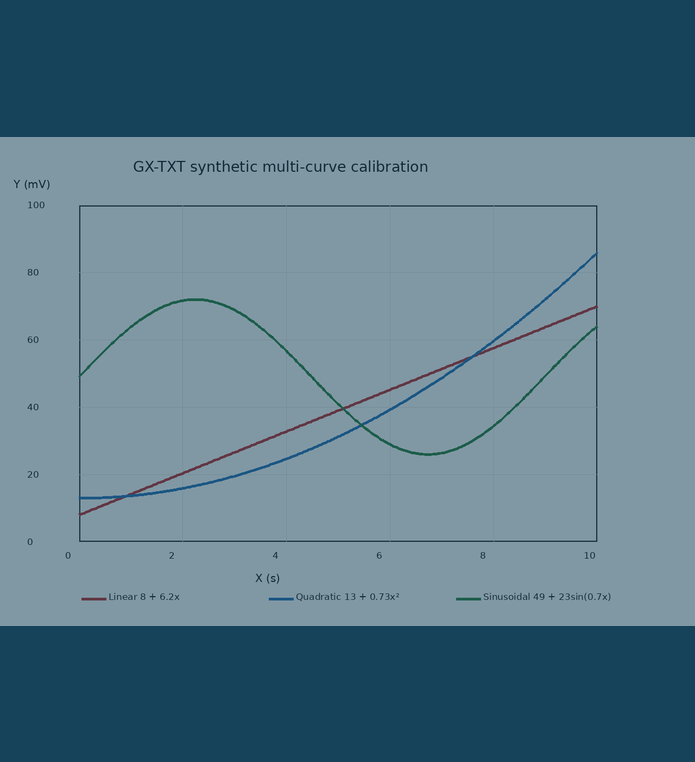
The values 45 and #17435a were entered without pressing Apply. The dialog shows Changes not applied; the Workspace still keeps opacity 100 and background #303030.
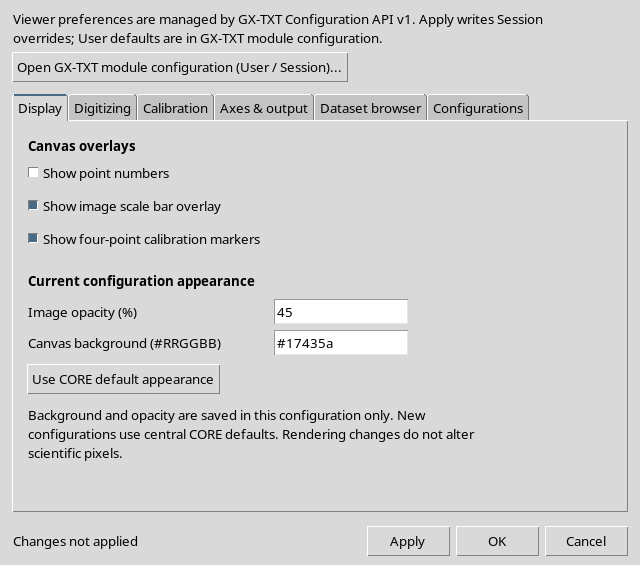
Pressing Cancel discards the draft without changing the canvas appearance or the persistent record.
11. Apply and Raster Customization
Repeating the same operation and pressing Apply, the footer shows Applied and saved to the selected configuration. The settings window stays open.
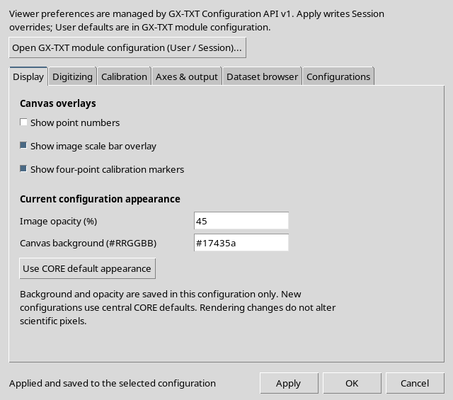
The native Workspace has now taken on Image opacity = 45 and Canvas background = #17435a, with the same source Dataset and the same SHA-256. The figure becomes fainter, while the three traces and their pixel positions remain visible.
The Digitizer Configuration is persistent, but this is not a change to the framework User defaults.
12. Opacity at 0%: Hidden Figure, Not a Missing Dataset
Setting Image opacity (%) = 0 and applying the change, the canvas becomes uniformly the chosen color #17435a.

The image, however, had not been deleted. Source information still indicated v05.synthetic_multicurve, the Dataset is present in the registry and the SHA-256 digest is unchanged.
This distinction is practical: if the canvas looks empty but the source is still associated, first check the opacity and the zoom scale, rather than automatically interpreting the visual absence as SOURCE MISSING.
13. Restoring with Use CORE default appearance
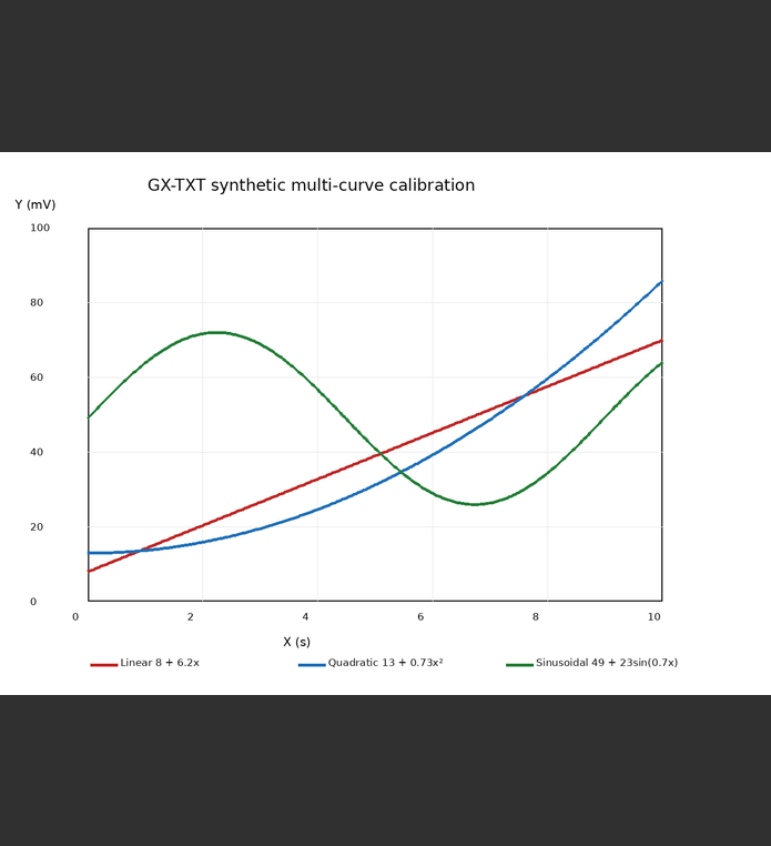
The Use CORE default appearance button fills the draft with the appearance values resolved from the central configuration. In our case it proposed 100 for opacity and #303030 for the background color.
After Apply, the raster became visible again in its original rendering; here too the Dataset was neither recreated nor modified.
The restoration of the local value must not be confused with clearing the CORE overrides: the appearance is saved in the configuration, and the effective User/Session value may have a different origin. Guide V03 covers the User and Session scopes in detail.
14. Overlays: What the Three View Commands Show
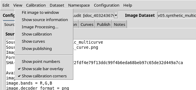
The View menu offers three check options:
| Label | Function |
|---|---|
Show point numbers | Show the indices of digitized curve points |
Show scale bar overlay | Show the saved scale bar |
Show calibration corners | Show the calibration corners |
15. CORE, Workspace and Saving the Overlays
The checkboxes in the View menu immediately write the shared preferences to the CORE Session. The scientific configuration also keeps a copy of the presentation flags in its own Workspace.
Here is the actual cycle: after the checkboxes were changed, the CORE reported the new values but the document had not yet been saved. Requesting to close the Viewer brings up the Save changes before Close? window, with Yes, No and Cancel.
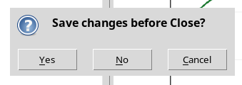
- Cancel: the window stays open and the draft change is kept.
- Yes: saves the new flags in the Workspace before closing.
16. Resizing the Window Without Losing the View
The Viewer window is made smaller. The canvas went from 695 × 763 to 555 × 703 pixels, but the Workspace kept exactly the same scale and the same offsets.
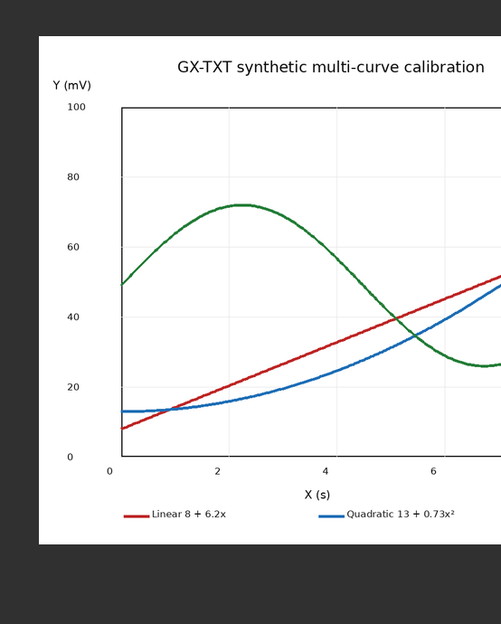
Ordinary resizing does not automatically perform a Fit and does not cancel the zoom chosen by the user. If after resizing it is important to see the whole image again, use View → Fit image to window explicitly.
17. Saving and Restoring Zoom/Pan
The non-default view is recorded in the Workspace through the Viewer’s ordinary update. If the window is closed normally and then reopened with the actual GX-TXT Digitalizer panel, the scale, X offset and Y offset match the saved values, as do the source Dataset, the overlays returned to their initial state and the canvas appearance.
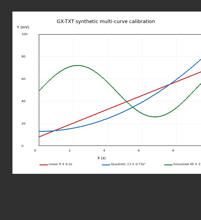
The framework distinguishes the view parameter from the scientific changes relevant to the Save/Discard check: zoom and pan can be persisted without being considered curve changes. This does not, however, prove that a sudden exit before the scheduled save will always preserve the last movement. Full handling of crashes, Session changes and recovery belongs to guide V27.
18. Verified Final State and Data Origin
At the end of guide V05, View → Fit image to window was invoked again, returning the window to the initial view with opacity at 100%, background #303030 and overlay checkboxes OFF / ON / ON.
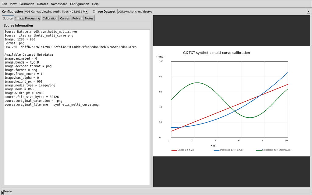
The Show point numbers, Show scale bar overlay and Show calibration corners preferences were saved and restored only in the context of the synthetic Session. The User defaults and other GX-TXT installations were not modified.
19. Limits, Distinguishable Problems and Deferred Checks
Apparently empty canvas. This can be caused by 0% opacity, minimum scale or a very large pan, not necessarily by loss of the source. Check Source information, the opacity and Fit image to window.
Very strong zoom. At the maximum scale of 50× the canvas displays a tiny region of the raster, with evident visual interpolation. This does not mean the source contains new high-resolution data.
Invisible markers. The overlay checkboxes do not create points, a scale bar or calibrated corners. The graphic effect may be nil in a configuration that lacks these objects.
Right-click. In Source it allows panning by dragging; in Curves it can open a context menu when the cursor meets a recognized point. The complete point-editing behavior is deferred to V13/V18.
20. Operational Summary
To work on the figure: use the wheel to zoom around the pointer, the middle button or right-dragging away from points to pan, and View → Fit image to window to see the whole source again.
Use Configuration → Viewer settings… → Display for opacity, background and overlays. Use Apply to make the values effective, Cancel to discard a draft and Use CORE default appearance to restore the standard rendering. Save the configuration when you change display options that must survive a Workspace switch.
The essential distinction is that zoom, pan and canvas appearance change the presentation, not the coordinates or the identity of the scientific Image Dataset.