

Scientific Annotations, Notes and Viewer Preferences
Coordinates derived from a graph acquire scientific meaning only when they come with a reliable description of the source, the axes and the traces. In the GX-TXT Curve Digitalizer this information is handled in different places: scientific labels, configuration Notes, Dataset Notes and Viewer settings.
Their scope is not the same. Some preferences belong to the user or to the Session; other information belongs to the individual scientific document. The guide describes the actual controls, how to save changes and how to check that none of them accidentally alters the digitized points.
1. Telling the Source Apart from the Documentation
The example uses a synthetic image with a dark trace, a second pink stroke and a grid. It was imported as the original Image Dataset into the framework Session.
The image measures 1280 × 900 pixels. Its colors, marks and thickness are not automatically experimental measurements or uncertainty estimates.
2. Creating a Stable Numerical Reference
The figure was calibrated with four corners: X from 0 to 10 s and Y from −20 to 80 mV. In the Curves tab ten manual points were placed on the dark trace.
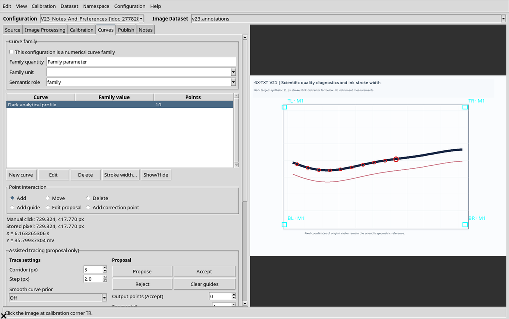
In what follows, titles, legend and display settings will be changed. To check that these are only descriptive changes, we will keep the same point_id values, raster coordinates and scientific coordinates of the ten points.
3. Entering Scientific Notes
Open the Notes tab. The main control is a UTF-8 text editor, suitable for describing the source, the meaning of the colors, any scanning distortions or deliberately excluded traces.
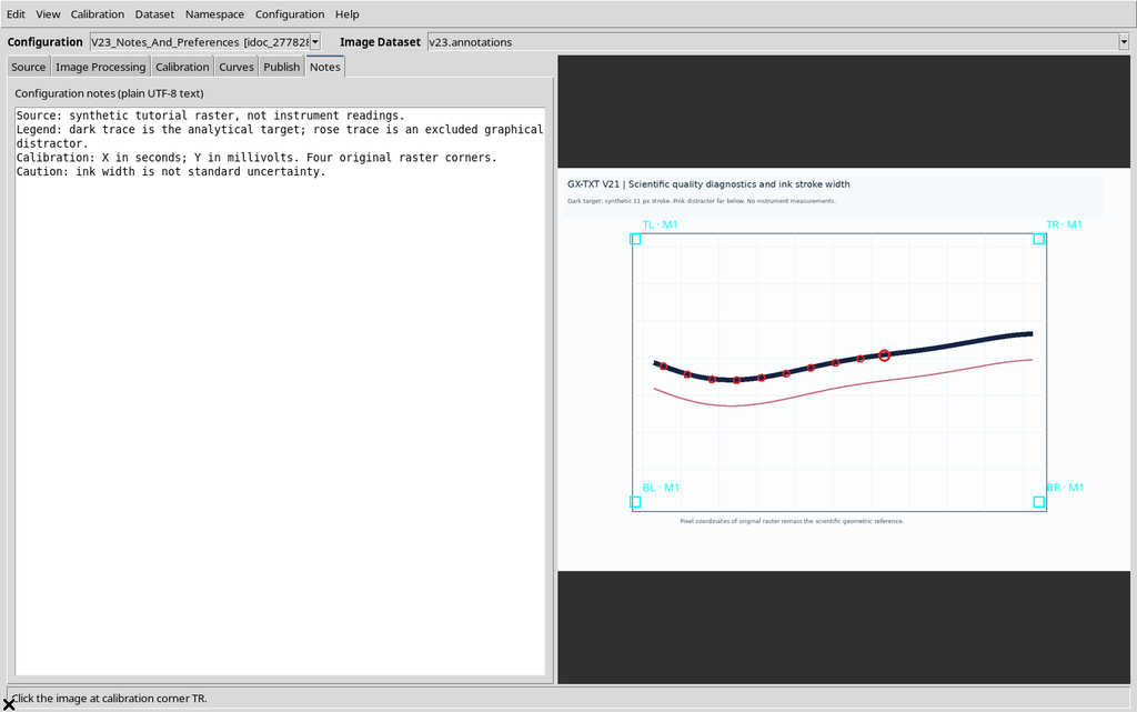
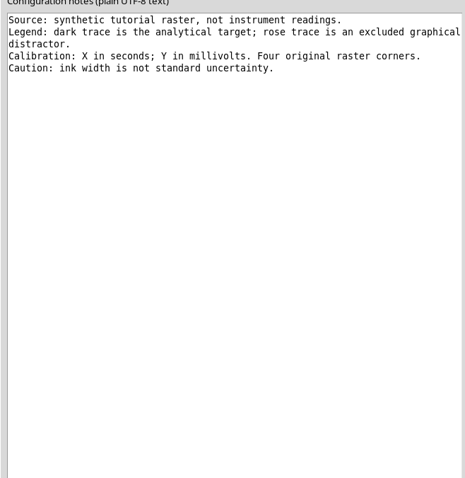
In our case we note that the dark trace is the object to be digitized, while the pink trace is a competing element. We also specify that the ink thickness does not represent a standard uncertainty.
4. Saving the Configuration Notes
When you leave the Notes field or switch to another tab, the Viewer can commit the changes through normal Workspace handling. For an explicit save choose Configuration → Save configuration.
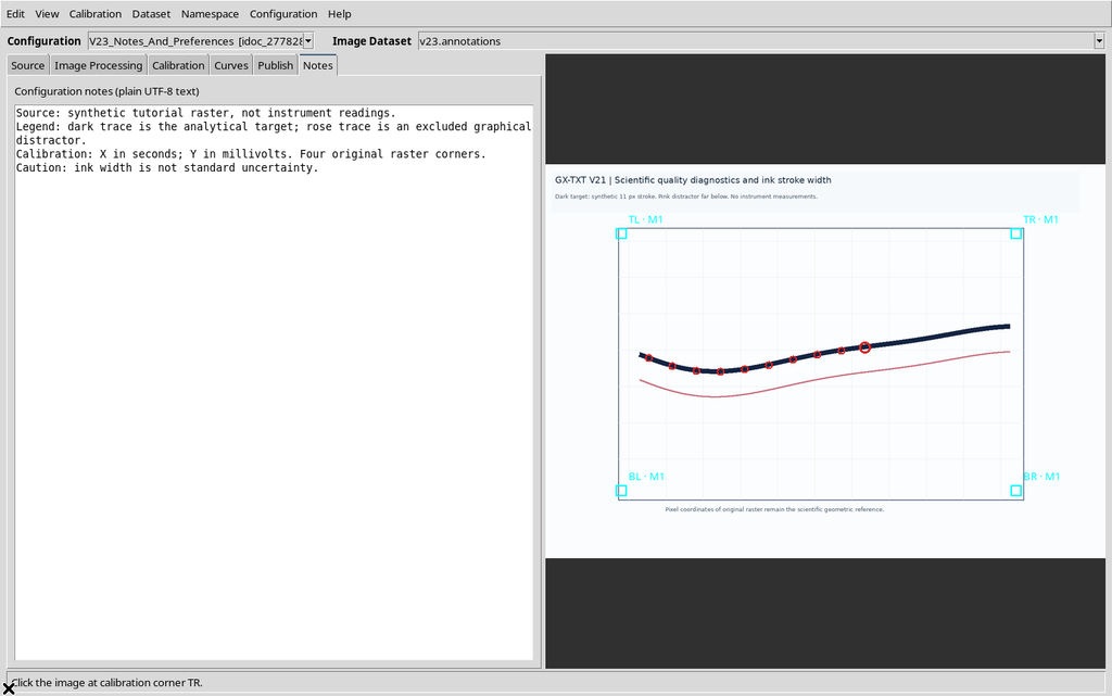
After leaving the editor and reopening it, the original text is still available. The Notes field does not add points, does not change the calibration and does not directly change the source Dataset.
5. Opening Viewer Settings and Telling the Preferences Apart
Select Configuration → Viewer settings…. The window has six tabs: Display, Digitizing, Calibration, Axes & output, Dataset browser and Configurations.
The commands in the Display tab change what is shown, not the scientific content of the image.
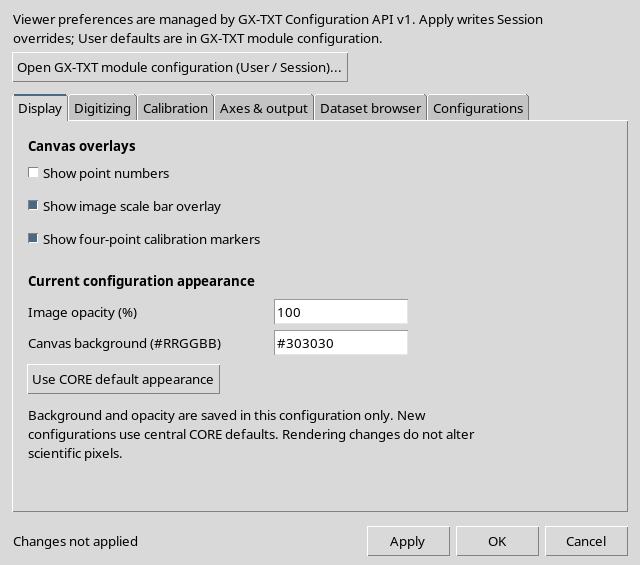
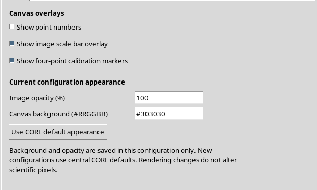
The window also brings together some shared framework preferences and some local values of the active configuration. The distinction becomes clear after Apply.
6. Digitizing: Selection and Ordering
The Digitizing tab contains Snap to darkest pixel, its radius, the monotonicity preferences, the point order and the number of points for the next assisted acceptance.
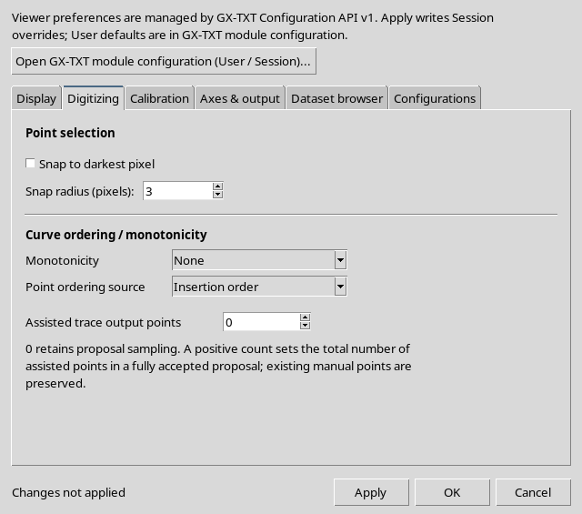
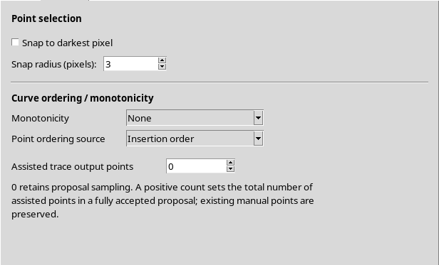
A snap set now applies to future insertions or moves that use it. It does not retroactively reposition the ten points already acquired and does not change their UUIDs.
7. Calibration: New Default Values
The Calibration tab lets you choose the convention for scale bar ticks, the Y direction of the full-image calibration and the default values for new measurements.
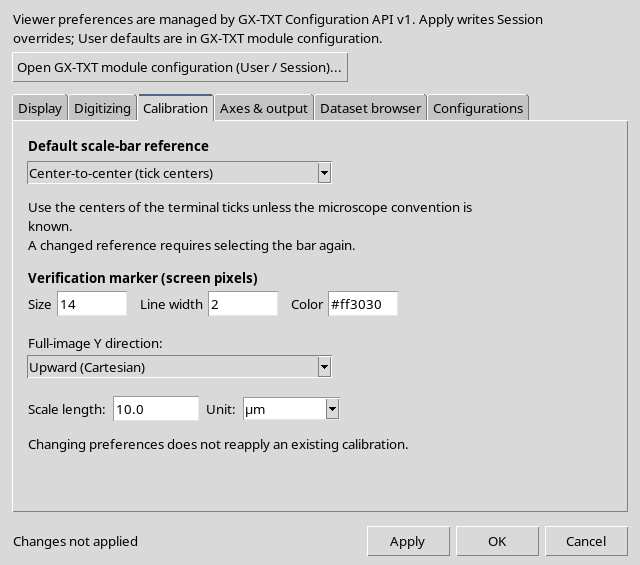
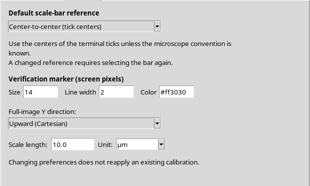
The verification marker fields are Size, Line width and Color. These are visual parameters for later verifications, not the metrological accuracy of the calibration. If the current scientific scale has already been accepted, these new defaults do not automatically transform it.
8. Axes & Output: Identity and Name of the Result
The Axes & output tab shows a summary of the current axes and lets you prepare the Output Dataset identity, the visible name and the naming template.
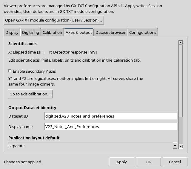
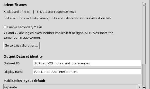
The base ID, the description and the Dataset naming template will be used in a future publication. Saving them is not the same as publishing a Dataset. Limits, units and scientific calibration are edited in the Calibration tab.
9. Dataset Browser: Catalog, Namespaces and Refresh
The Dataset browser tab handles the search for Image Datasets and the catalog refresh options.
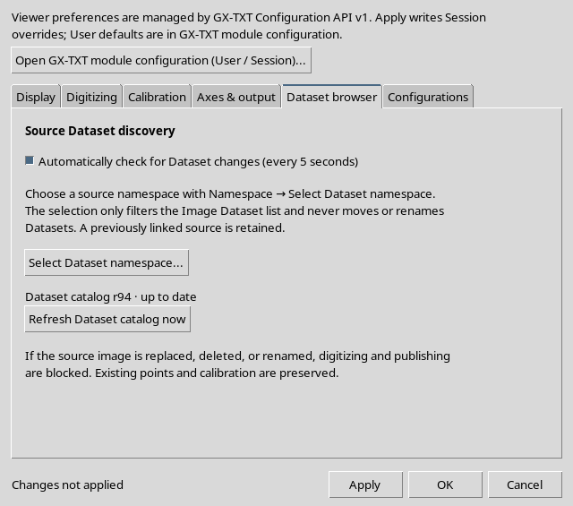
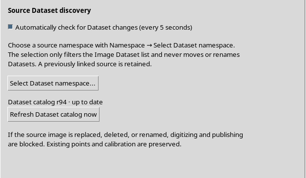
Turning off the automatic check or refreshing the catalog manually does not move files and does not change the ID of the source already associated. The namespace selector filters what is shown.
10. Configurations: Several Documents in the Same Session
The Configurations tab lists the scientific documents saved in the Session.
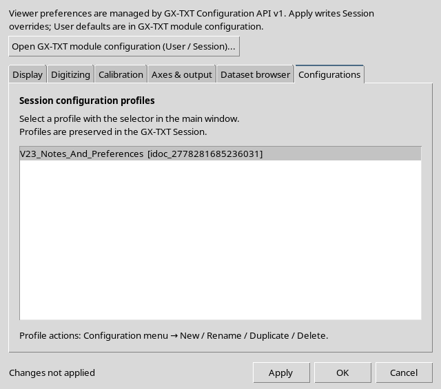
To open, rename, duplicate or delete a configuration, use the selector and the Configuration menu in the main window. Each document has its own identity; two configurations can use the same image without necessarily sharing all the annotations.
11. Unapplied Changes: Cancel
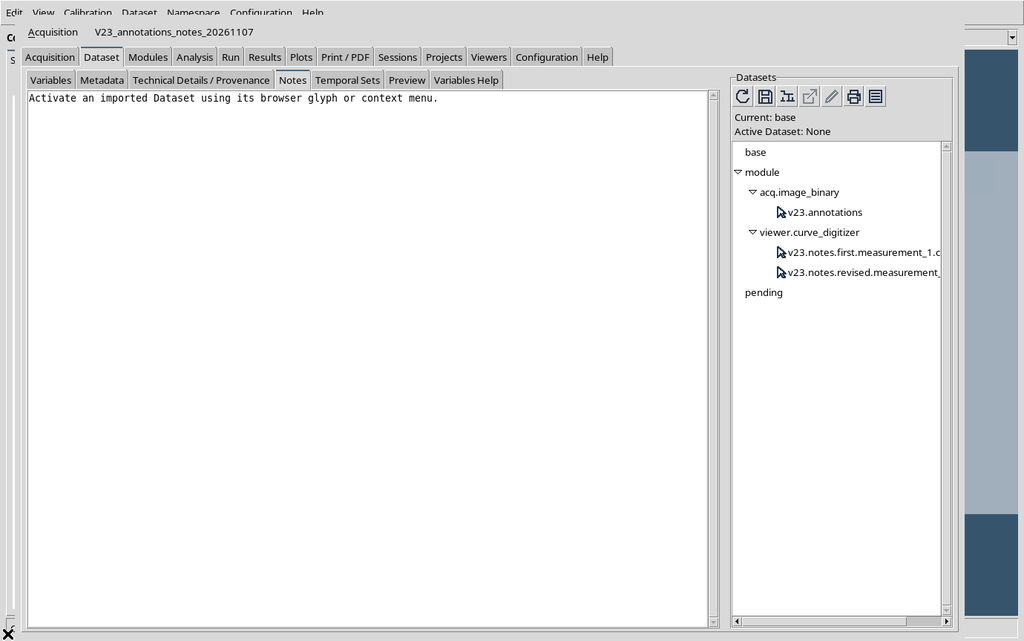
Before saving, we temporarily change Show point numbers, Image opacity and Canvas background, then press Cancel.
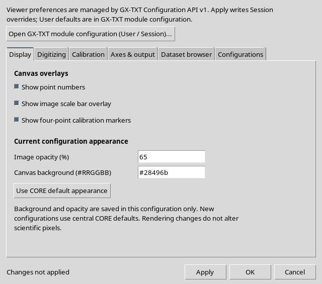
Reopening the window, the previous values still appear.
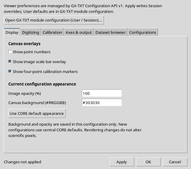
Cancel discards the unapplied changes: it does not partially save the preferences and does not alter the scientific document.
12. Validation: Snap Radius Out of Range
In the Digitizing tab we try to set Snap radius = 26.
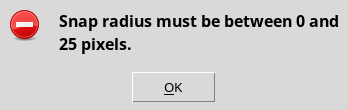
The Viewer rejects the request because the allowed range is 0–25 pixels. The settings are not partially applied: correct the value and repeat Apply, without assuming that the other fields were saved.
13. Setting a Valid Radius
We set Snap radius = 4 and enable Snap to darkest pixel.
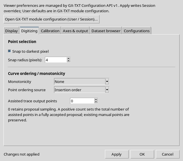
The choice concerns the selection of future points, not the accuracy of the data already digitized. When there are several lines, an unchecked snap can latch onto the wrong trace: always check the new point on the raster.
14. Default Values for Future Calibrations
In the Calibration tab, as an example, we choose Outer edges of ticks, Downward (image pixels) for the next full-image calibration, a new scale reference of 25 mm and a verification marker with Size 16, Line width 3 and Color #2aa5d4.
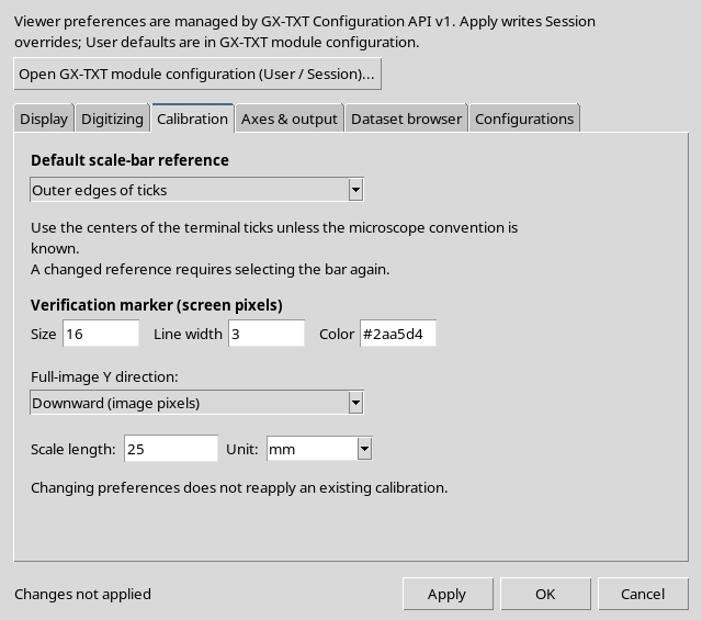
Choosing a new default does not mean that the current image contains a 25 mm scale bar. The four-point calibration already accepted still represents the limits from 0 to 10 s and from −20 to 80 mV.
15. Local Appearance of the Configuration
In Display we turn on the point numbers, temporarily hide the scale and corner overlays, and choose Image opacity = 72% and Canvas background = #20394a.
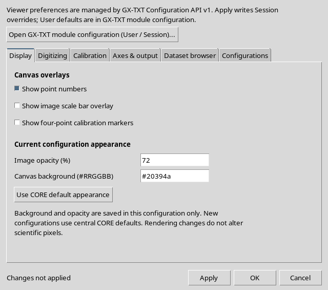
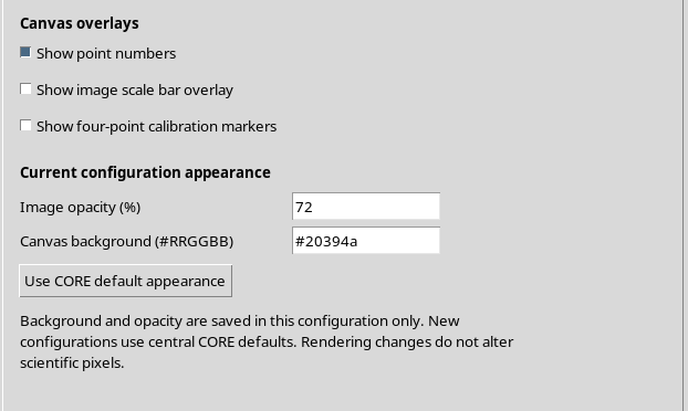
These appearance values are stored in the current scientific configuration. The original raster is not recolored and the numerical data are not rewritten.
16. Preparing Name and ID Without Publishing
In Axes & output we set an example ID for the next publication and a description that identifies the synthetic curve.
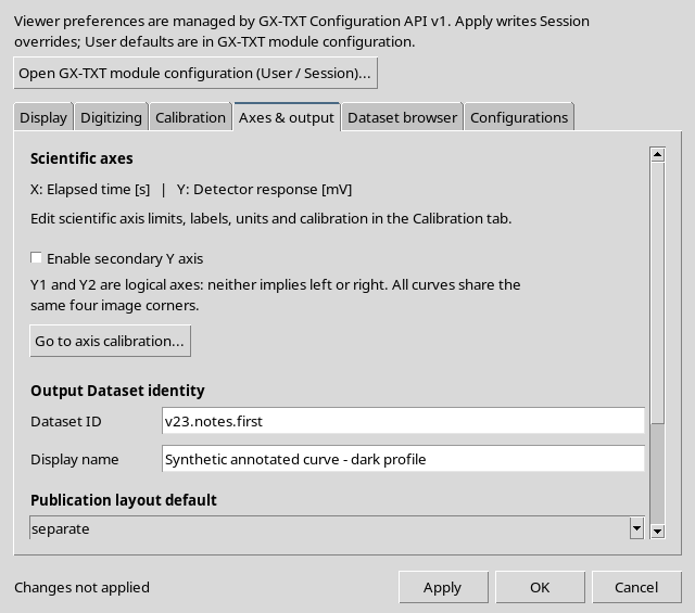
The Dataset ID is not the name of the configuration: the latter holds the state of the work, while the published Dataset will be a standalone object. A new ID can be used to publish a later version of the notes, keeping the same numerical geometry.
17. Manual or Automatic Catalog Refresh
The Automatically check for Dataset changes control can be turned off temporarily while working.
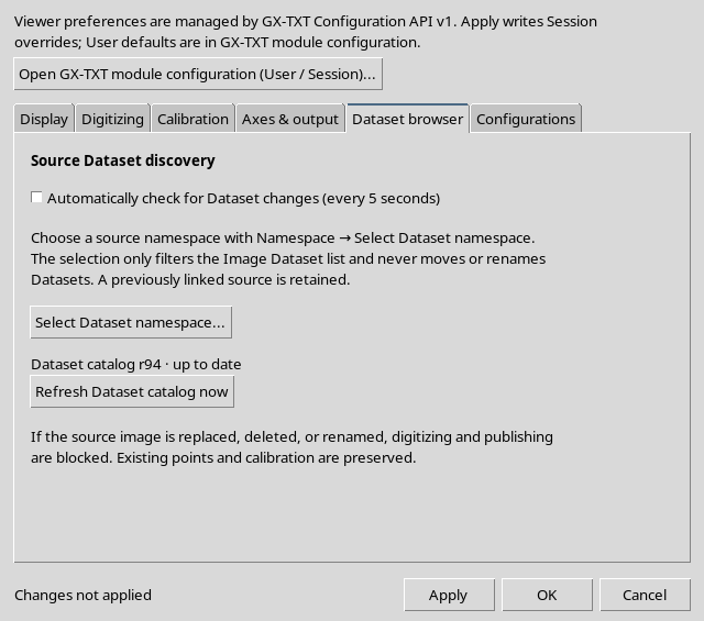
A manual refresh with the Refresh Dataset catalog now button updates the selection options; it does not change the current image. Automatic mode was later re-enabled in the example Session.
18. Apply Saves and Leaves the Window Open
We press Apply with all values valid.
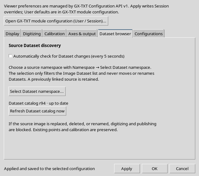

The window stays open and shows the result of the save. A second Apply can save again using the updated CORE state. OK applies and closes; Cancel closes without applying any new changes left in the draft.
19. User Defaults, Session Overrides and Configuration
The same setting can come from several levels. The CONFIGURATION_API_v1 distinguishes:
| Scope | Owner | Example |
|---|---|---|
| User defaults | Personal default values of the module | Show point numbers initially disabled |
| Session override | Preference shared within the open Session | Show point numbers on; Snap radius 4 |
| Configuration document | Scientific property of the specific document | Notes, curve name, opacity 72%, background #20394a |
The User defaults values stay unchanged. The shared preferences updated with Apply are kept as Session overrides, while the Canvas appearance stays associated with the scientific configuration.
The framework uses the precedence order of the configuration levels; a Session override must not be confused with a global change for the user.
20. Numbers and Overlays: Representation Only
After applying, in the Curves tab we see the point numbers and the new Canvas rendering, while some calibration markers are hidden.
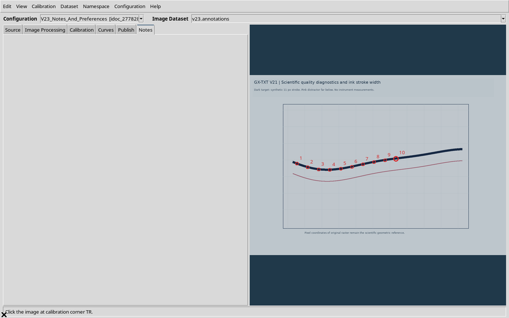
These options change the visible symbols, not the order and coordinates of the numerical table. The distinction matters when taking screenshots for scientific documentation.
21. Changing the Name of a Curve
In the Curves tab, select the series and press Edit to open the native dialog.
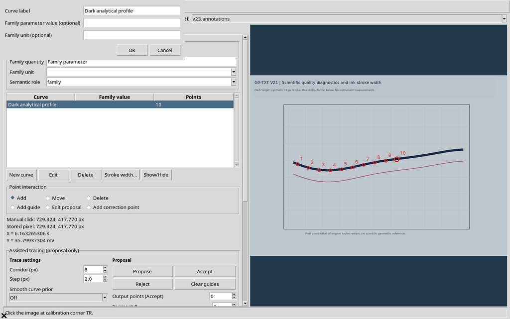
We enter a more descriptive name that clarifies the interpretation of the trace.
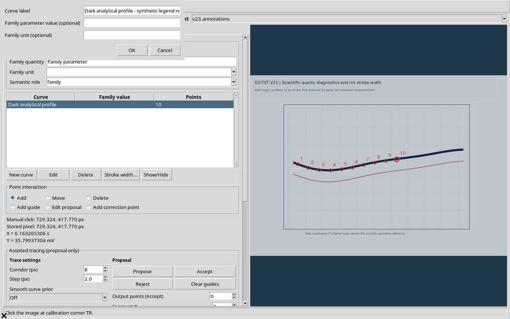
After OK, the new name appears in the list.
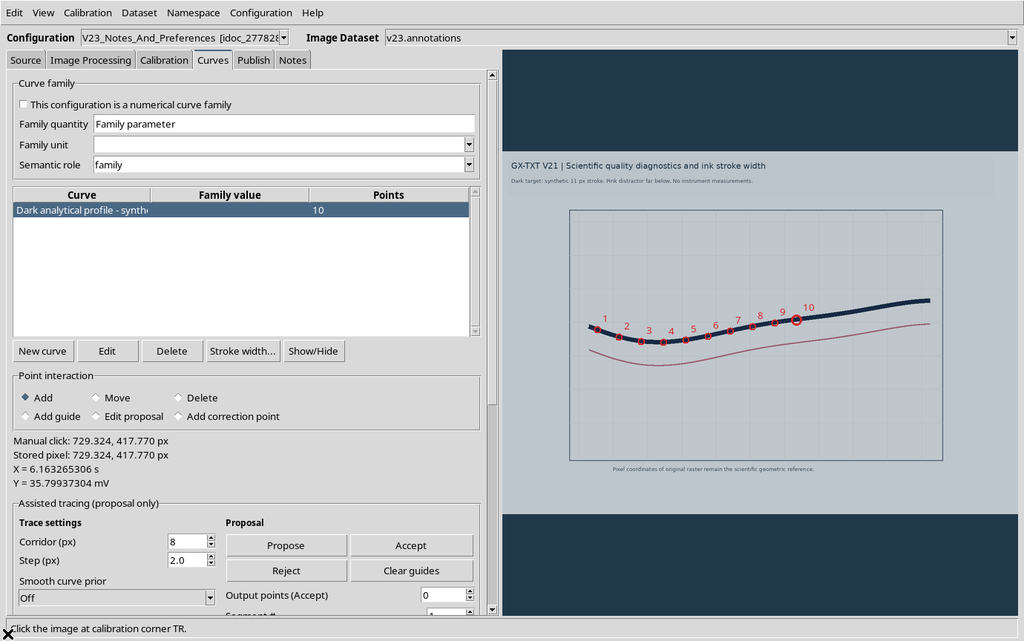
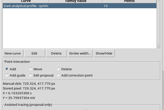
The name is part of the scientific context, but it does not alter the ten point_id values or the saved coordinates.
22. Changing the Axis Labels
We switch to Calibration. Before the change, the axes are identified as Elapsed time and Detector response.
We change only the names to Elapsed time since trigger and Synthetic detector signal, then press Apply axis settings.
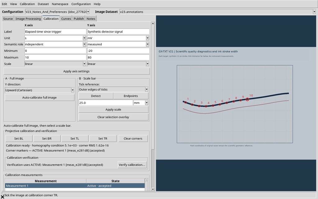
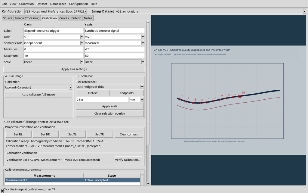
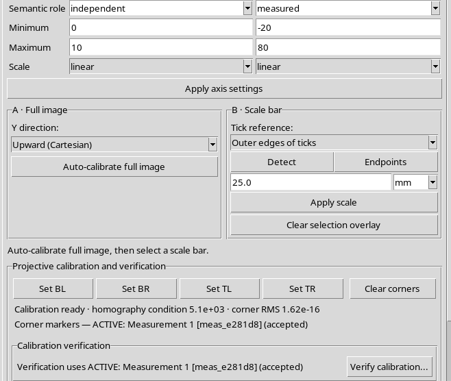
The units s and mV, the limits and the four corners stay identical. The comparison of the records confirms that the scientific coordinates and the identifiers of the ten points are also unchanged. Changing a label is not the same as changing a scale.
23. Checking That an Annotation Is Not a Transformation
The check can be summarized by distinguishing the fields that were changed from those that were kept.
| Element | Result |
|---|---|
| Curve name | Updated |
| Axis names | Updated |
| X/Y units and limits | Unchanged |
| Four-corner calibration | Unchanged |
| Original raster | Unchanged |
| Ten UUIDs and scientific points | Unchanged |
If limits, units or transformation were changed instead, the new meaning of the data would have to be checked. This guide concerns only descriptive annotations.
24. Publishing a First Version with Notes
In the Publish tab we choose the accepted calibration and a new ID.
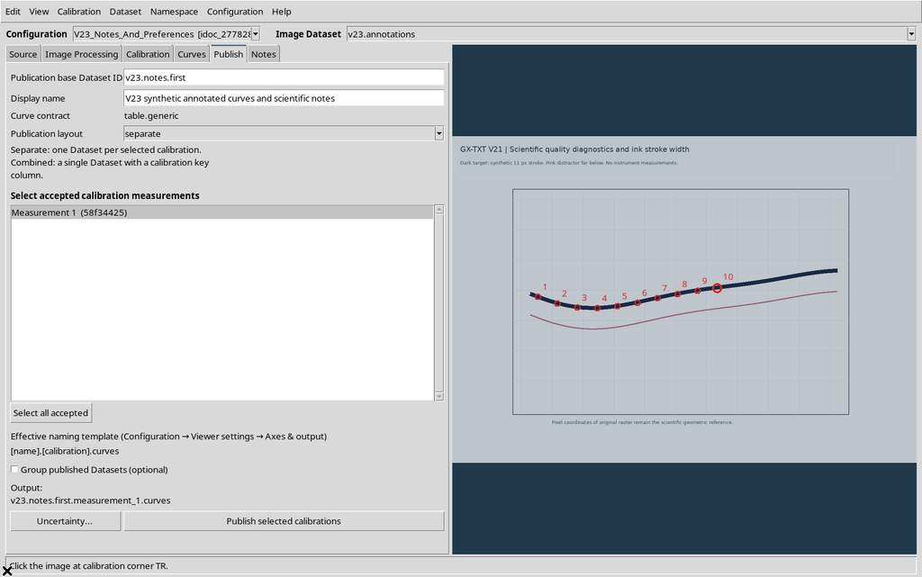
Publishing creates the numerical Dataset with the ten points and links the notes present in the configuration.
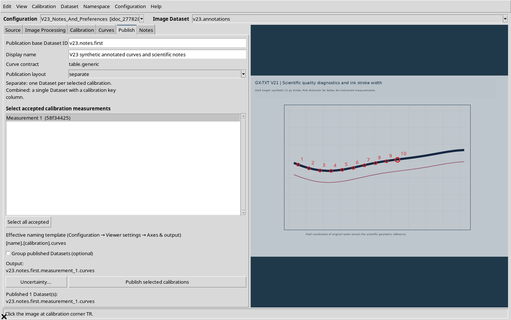
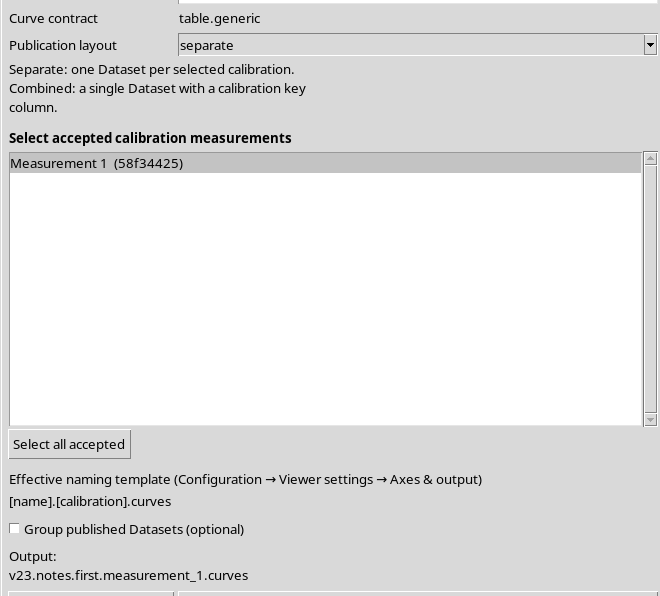
The notes are saved as a Dataset Notes Markdown document, not turned into new numerical columns. The descriptive name of the Dataset and the structured metadata keep a distinct role.
25. Revising the Legend in the Notes Tab
After checking the source, we edit the text in Notes to state that the pink trace does not belong to the selected curve.
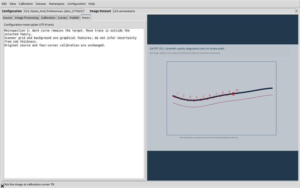
The revision is saved through FocusOut and Configuration → Save configuration. The text does not change the number or position of the points.
26. Publishing a Second Dataset with the Revised Notes
To keep the later documentation as well, we prepare another Dataset ID, keeping the same calibration.
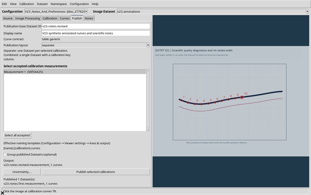
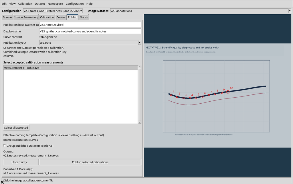
The result still contains ten points: the canonical table has the same numerical bytes and the same SHA-256 as the first publication, because the coordinates were not changed.
27. Numbers and Documentation Are Not the Same Thing
The two publications contain the same coordinate table but two different notes documents. The first keeps the initial context; the second contains the revision.
It is therefore possible to have the same numerical identity of the content, but different Dataset identities and documentary content. For this reason the author must keep the references to the source, the points and the version of the notes without confusing them.
28. Opening Dataset Notes from the CORE
From the GX-TXT menu we open the native Dataset notes… button and select the first Dataset.

The control is in the common GX-TXT environment. It is not a second scientific editor of Curve Digitalizer: it lets you read the Markdown document associated with the canonical Dataset.
29. Markdown Source and Formatted Preview
The CORE shows the notes editor in the Dataset tab, with GX-Markup / Markdown source and Rendered preview.
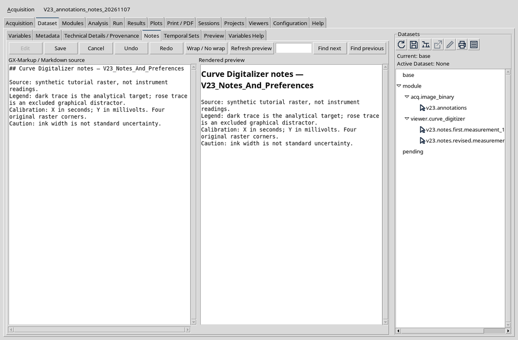
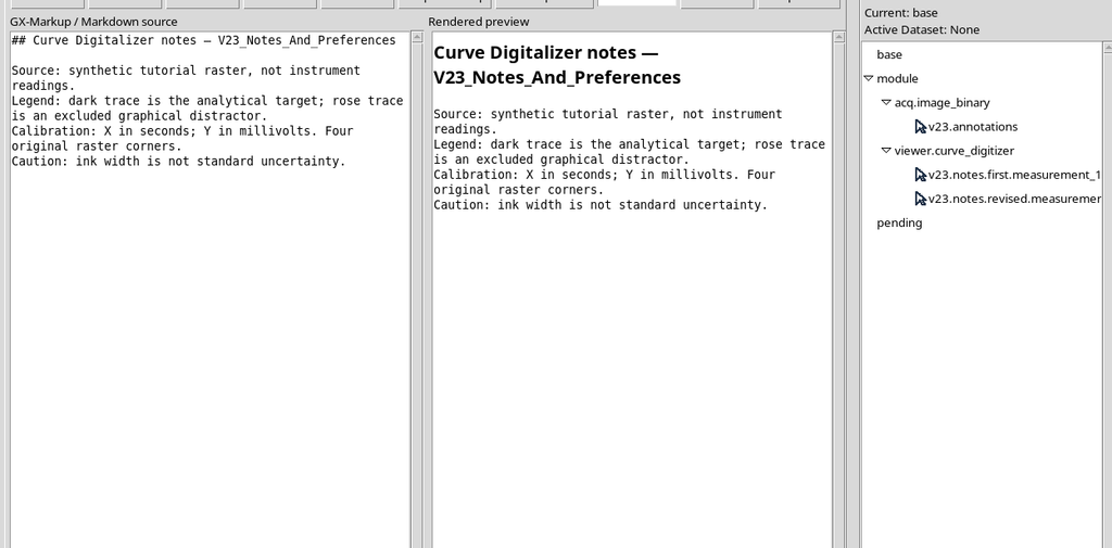
The published text keeps the section titled with the Curve Digitalizer Notes. Its references to the image and the legend can be read without opening the original interactive document.
30. Keeping the Previous Version Too
We select the second Dataset Notes. The CORE shows the revision of the legend.
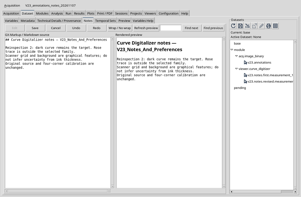
The two documents have different content and were verified as separate Markdown files. Viewing them and choosing Cancel, no rewrite takes place. The notes of the first publication stay available alongside the second.
31. Duplicating a Scientific Configuration
The Configuration → Duplicate configuration menu creates a copy with a new configuration identifier.
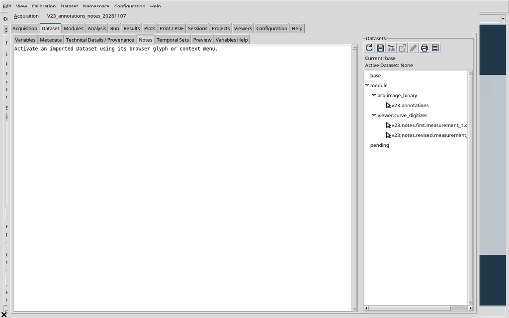
In this example the copy keeps the source and the ten points, but receives a new identity for the calibration group and its realization. Duplication does not automatically publish a further numerical Dataset.
32. Independent Notes in the Copy
We open the Notes of the copy and enter an alternative explanation, referring to the same synthetic image.
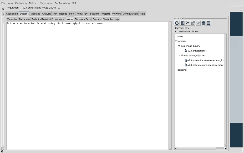
The text belongs to the new document. Going back to the original configuration, its prose is not replaced by that of the copy.
33. Independent Appearance for the Copy
In the copy we set Image opacity = 54% and Canvas background = #36556c.
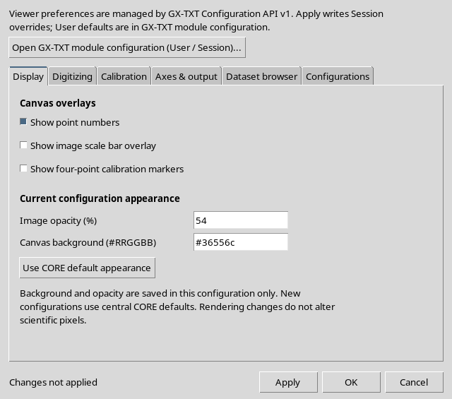
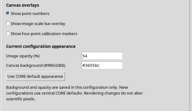
After Apply, the copy document keeps its own appearance and its own notes.
The shared Session preferences, instead, keep applying to both documents; we did not change the User defaults.
34. Going Back to the Original Configuration
From the selector at the top we resume the original configuration.
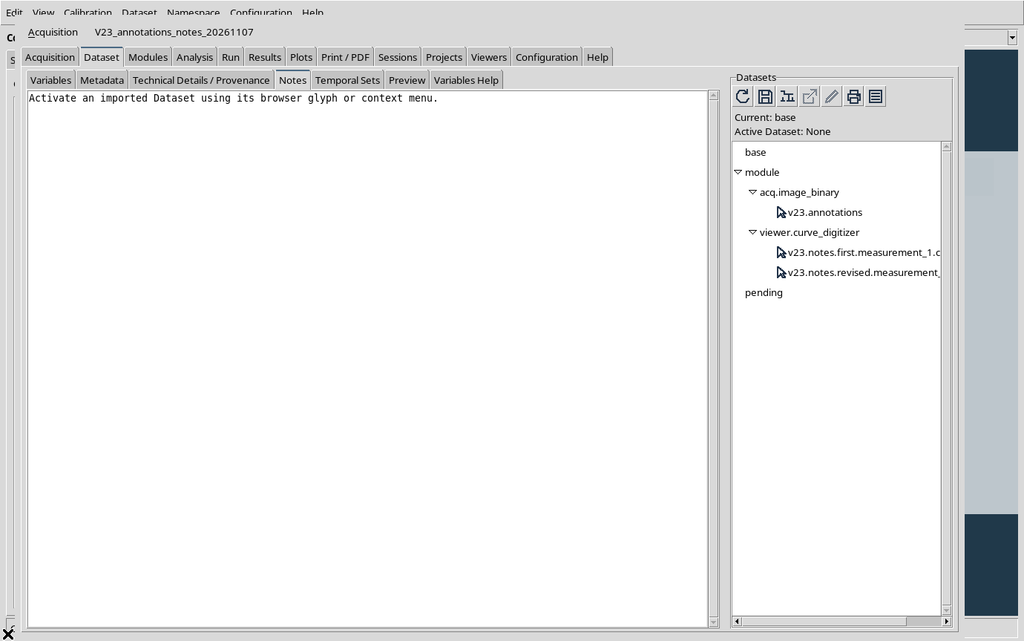
Its revised Notes, the opacity of 72% and the background #20394a are recovered. No change made to the copy propagated to the text or appearance of the original.
35. Save, Close and Reopen of the Notes
We save the configuration, close the Viewer normally and reopen it from the same Session.
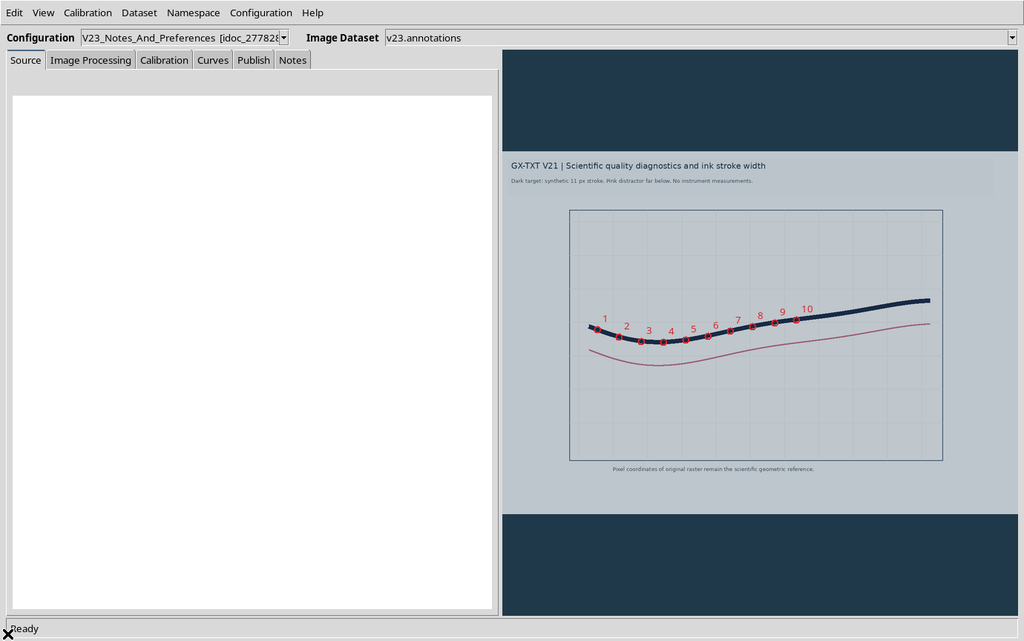
The text in Notes is still present. The original Dataset and the two published Markdown documents are persistent as well. The persistence of the interactive document is distinct from the persistence of the canonical tables already published.
36. Checking the Saved Display After Reopening
In the original configuration the Display tab still shows the selected appearance values.
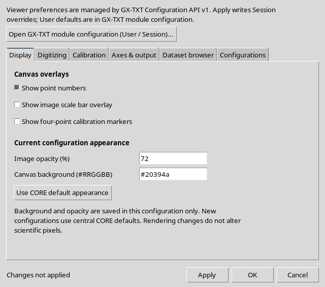
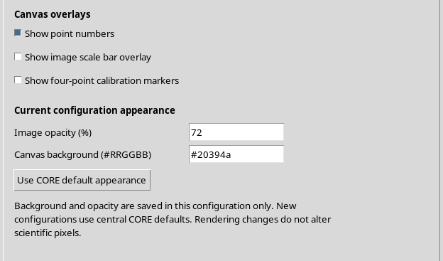
The opacity of 72% and the color #20394a are per-configuration. Another configuration in the same Session can use different ones without changing the global defaults.
37. Checking the Shared Preferences
The Digitizing tab still shows snapping and its radius of four.
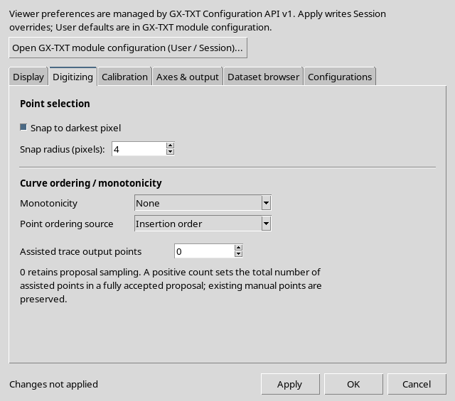
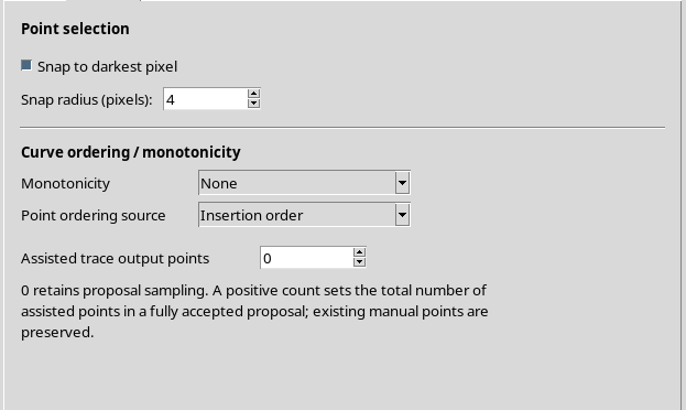
These shared settings come from the Session in the Configuration API. The same preferences are therefore available when switching to the copy; the notes and the Canvas color, instead, stay specific to the document.
38. Calibration and Dataset Browser After the Restart
In the Calibration tab the new defaults for later actions are available, without changing the original calibration.
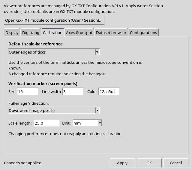
In the Dataset browser a manual catalog refresh can be requested, keeping the associated source.
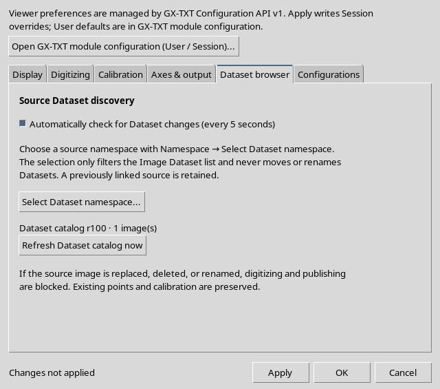
A browser setting is not a change to the points or to the physical provenance of the raster.
39. Checking the Points Again
The Curves tab displays the ten acquired points with the new names of the series and of the axes.
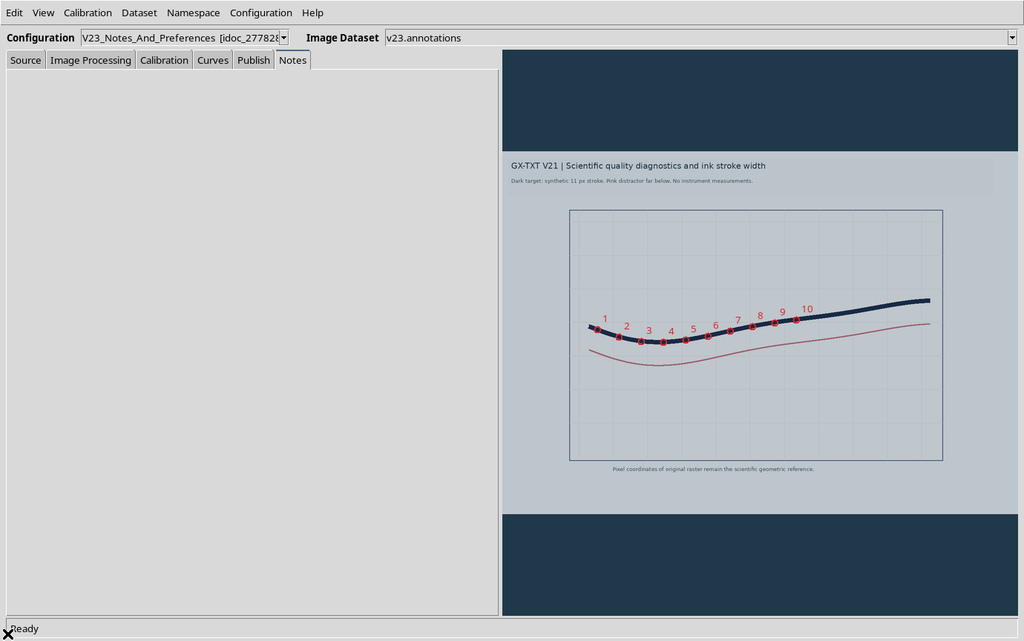
Checking the Workspace after Save/Close/Reopen confirmed the original identities and coordinates. Labels and display were rebuilt from the document without altering the scientific records.
40. Checking the Duplicated Configuration After Reopening
Selecting the copy, its Notes and its independent appearance are found again.
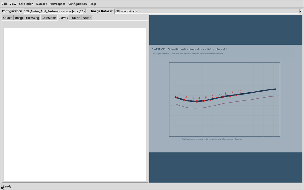
The original and the copy can be used for alternative scientific revisions, but their identifiers must be kept distinct, and they must not be presented as two independent experimental measurements when they are simply two interpretations of the same image.
41. Recommended Procedure and Limits
- Load an identified source and check its calibration before adding annotations.
- Give axes and curves scientifically meaningful names, without confusing the name with units or transformations.
- Enter in Notes the meaning of the traces and the precautions concerning the source.
- Use Viewer settings knowing how to distinguish User defaults, Session overrides and configuration-specific parameters.
- Check the field limits; a failed validation is not the same as a partial save.
- Use Apply to save without closing, OK to apply and close and Cancel to discard unconfirmed changes.
- Publish numerical Datasets with distinct identifiers; check the Dataset Notes documents separately.
- If the scientific context changes, keep a revision of the notes without automatically overwriting earlier publications.
- Duplicate a configuration when independent interpretations are needed, always distinguishing the new document from a new independent measurement.
- Save, close and reopen, then check points, notes, overrides, source and the documents associated with the Datasets.
Curve Digitalizer keeps measurements, scientific annotations, Viewer preferences and documentation of published results separate. This separation makes the work easier to understand, check and reproduce, but it does not automatically give the digitized data accuracy or metrological uncertainty.