

Scale Bar: Detection, Tick Conventions and Physical Units
This chapter (V06) describes the actual use of the Curve Digitalizer scale bar, from preparation to physical axes.
1. Source Pixels and the Scale Bar
A digital image initially contains coordinates in source pixels. A bar of known length can convert them into physical units, but only when its endpoints are correctly located and its length and unit are declared.
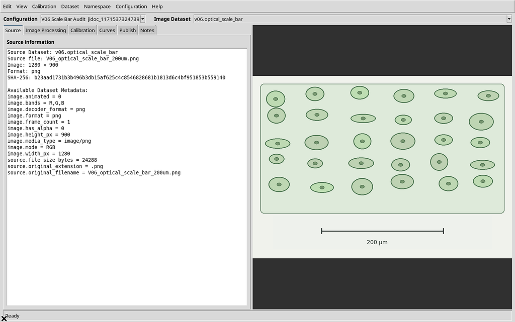
For chapter V06 a synthetic optical-microscopy scientific image was created (not a real micrograph) of 1280 × 900 pixels, with a horizontal bar and two vertical ticks. The distance between the tick centers is designed to be 600 pixels, and the label states 200 µm. This image is an input fixture, not an image of the interface; the following screenshots come exclusively from the running Viewer.
The raster was imported as a true canonical Image Dataset image.raster into the new Session used to create guide V06, and associated with a Digitizer Configuration. No numerical curve was published.
2. Mandatory Precondition: Auto-calibrate full image
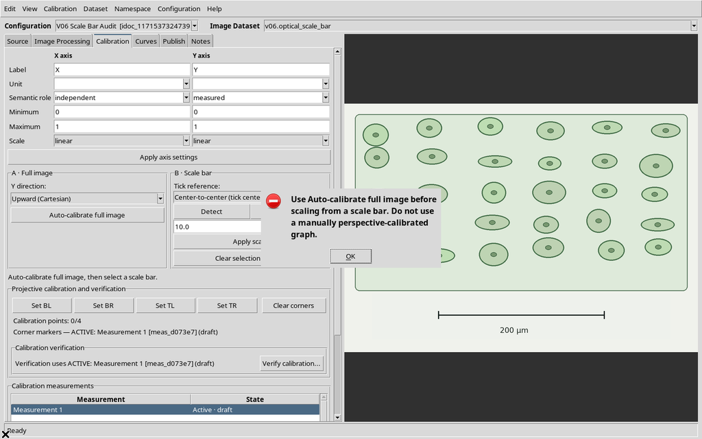
The physical scale function first requires the whole image to be calibrated. An attempt to use Calibration → Detect scale bar (click image) without this preparation is correctly refused:
Use Auto-calibrate full image before scaling from a scale bar. Do not use a manually perspective-calibrated graph.
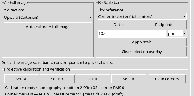
You need to open the Calibration tab.
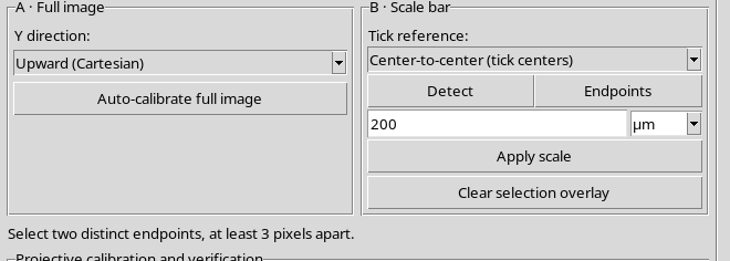
- The A · Full image section contains Y direction and Auto-calibrate full image;
- The B · Scale bar section contains Tick reference, Detect, Endpoints, length, unit, Apply scale and Clear selection overlay.
With Upward (Cartesian) and Auto-calibrate full image, the configuration acquires the four full-image corners, with the X axis from 0 to 1279 px and Y from 0 to 899 px. This step does not yet imply any physical length.
3. Guided Detection and Rejection of a Click Away from the Bar
Press Detect, then click on the horizontal stroke of the bar in the image on the right. The detector checks contrast and geometry near the chosen point; it is not a blind recognition of the whole figure.
A click deliberately placed far from the bar is rejected with:
No distinct horizontal scale bar was detected near the click. Use two endpoints.
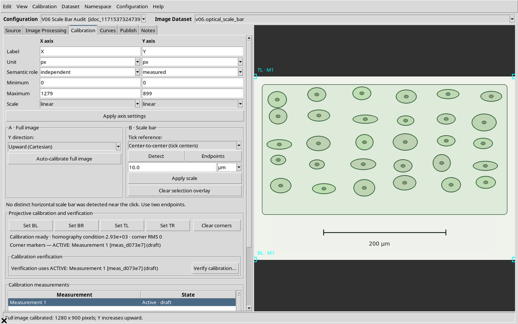
The rejection is not a fault: it prevents a segment not supported by the source pixels from being accepted. In difficult images, manual selection is the intended alternative.
4. Magenta Preview: No Measurement Applied Yet
Clicking on the center of the horizontal stroke, with Center-to-center (tick centers) selected, the GUI proposed a segment of 600 source pixels, drawn in magenta, with endpoints and the annotation Preview.
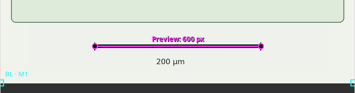
The state of the Workspace before and after the proposal still showed scale_reference = null and axes in px: the preview is not the applied physical calibration. A positive length, a valid unit and an explicit press of Apply scale are required.
5. Two Invalid Inputs Rejected by the GUI
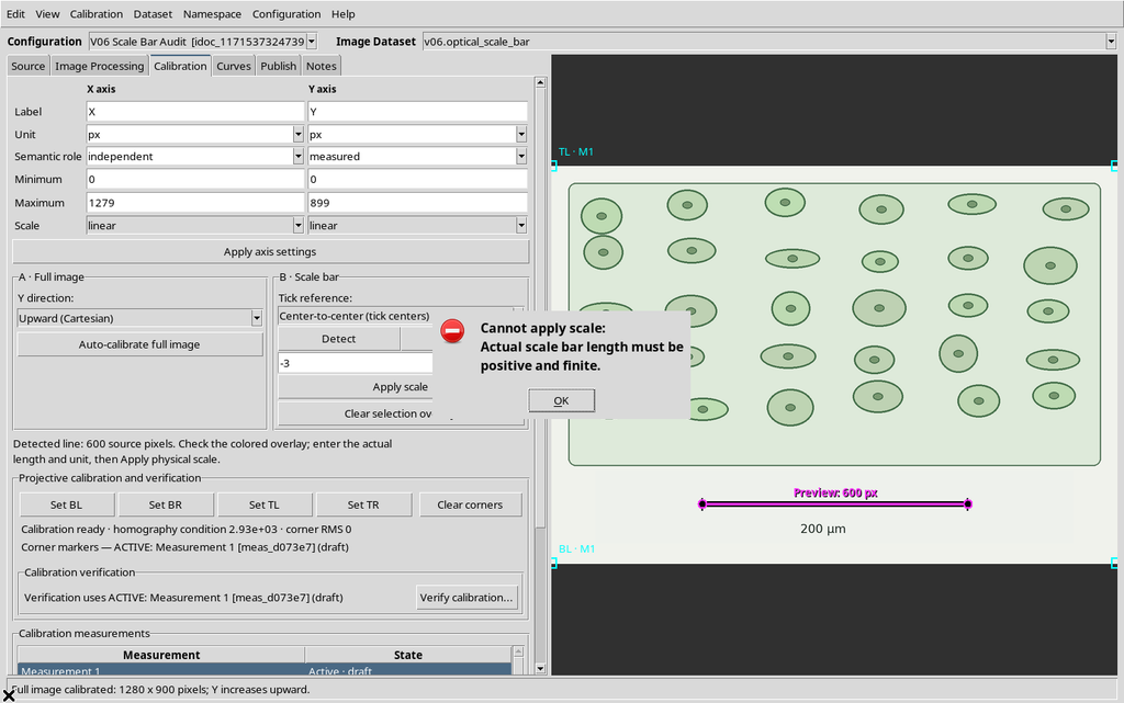
With a bar proposal pending, deliberately wrong values were entered.
With a length of −3 µm, Apply scale showed Actual scale bar length must be positive and finite.
With a positive length and an unrecognized unit, the Viewer showed Choose a recognized physical length unit.
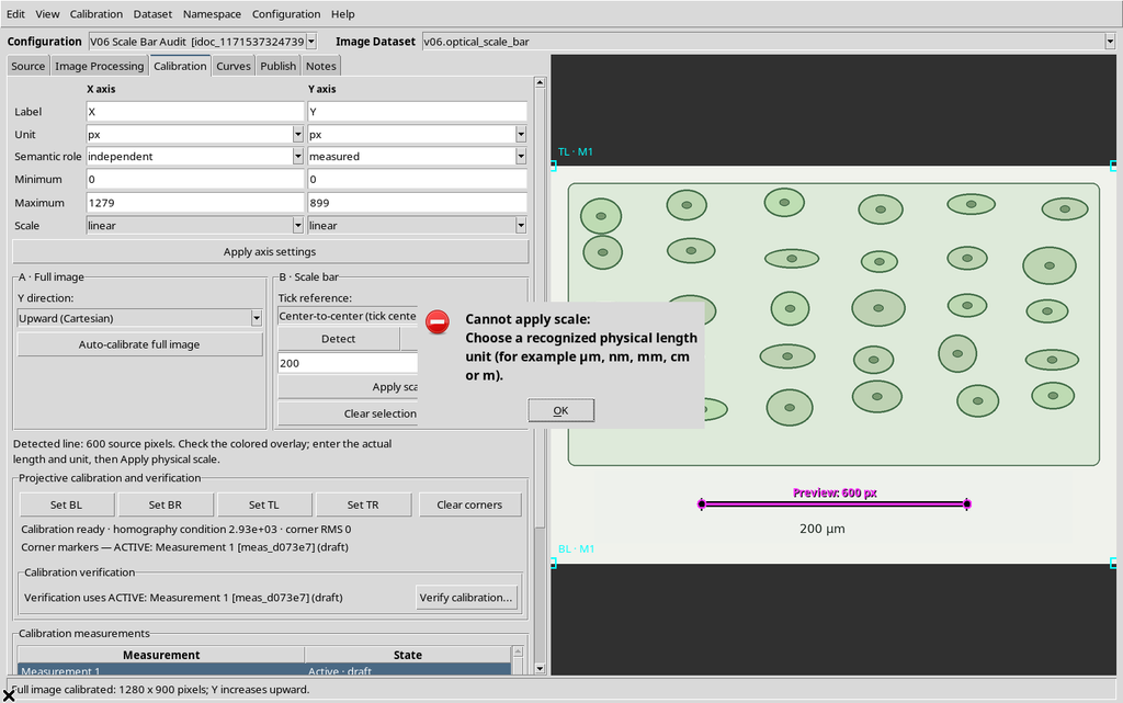
In both cases the document kept the axes in pixels, with no new physical reference. The supported units include µm, nm, mm, cm, m, pm, Å, um, μm, in and ft.
6. Physical Application: 600 px = 200 µm
Enter 200 in the length field and µm in the unit field; press Apply scale after checking the proposal. The Viewer recorded:
- Applied: 600 px = 200 µm
- 1 px = 0.3333333333 µm
The magenta line was replaced by the green line, with a black border, circular endpoints and the annotation 200 µm.
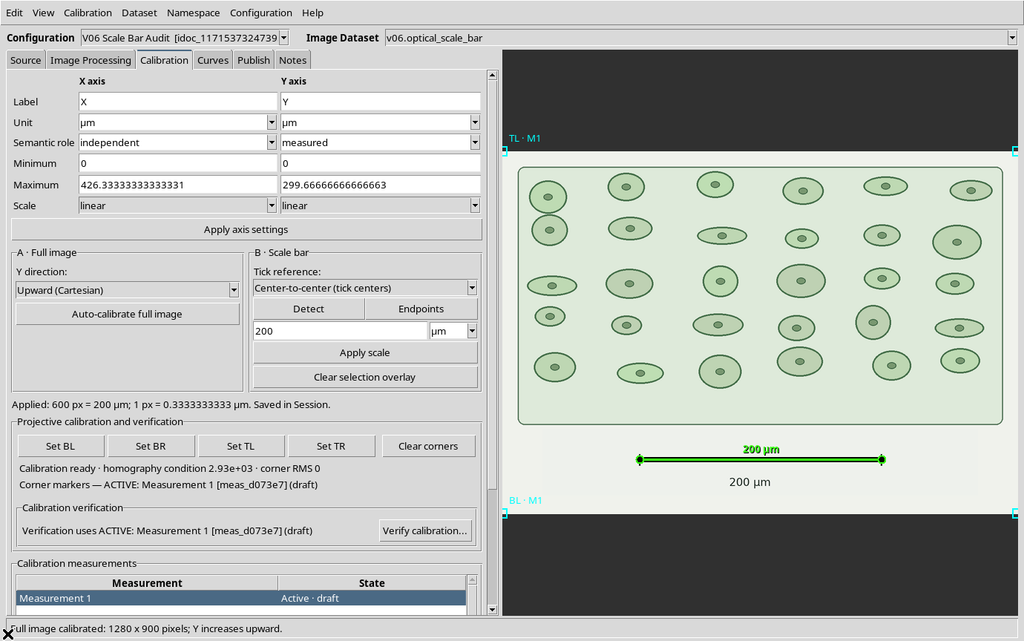
The factor is k = L / d = 200 / 600 = 1/3 µm per source pixel. Since pixel centers from 0 to W−1 and from 0 to H−1 are considered, the saved ranges are:
| Axis | Physical extent |
|---|---|
| X | 0–426.333333 µm |
| Y, Upward | 0–299.666667 µm |
The abundance of digits in the computed factor does not represent a measured experimental uncertainty.
7. Clear selection overlay Does Not Delete the Scale
Pressing Clear selection overlay makes the green line disappear from the view and the GUI states:
Scale overlay cleared. The applied calibration is preserved.
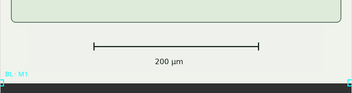
The Workspace, however, keeps the same scale_reference, the same endpoints and the same physical axes. Hiding an overlay is not the same as removing the calibration. The numerical reset is a different action, confirmed separately.
8. Changing Tick reference Invalidates the Proposal
The Viewer offers three geometric conventions: Center-to-center (tick centers), Inner edges of ticks, Outer edges of ticks. The choice cannot be made arbitrarily: you need to know whether the original bar refers to the centers or to the edges of the ticks.
To show the behavior, a second magenta proposal was prepared and Tick reference was then changed from center to inner edges. The proposal was invalidated, with the status Tick reference changed. Detect the scale bar again before applying.
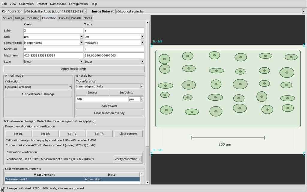
Pressing Apply scale without a new proposal, the Viewer refused the action with Select a scale bar on the image before applying.
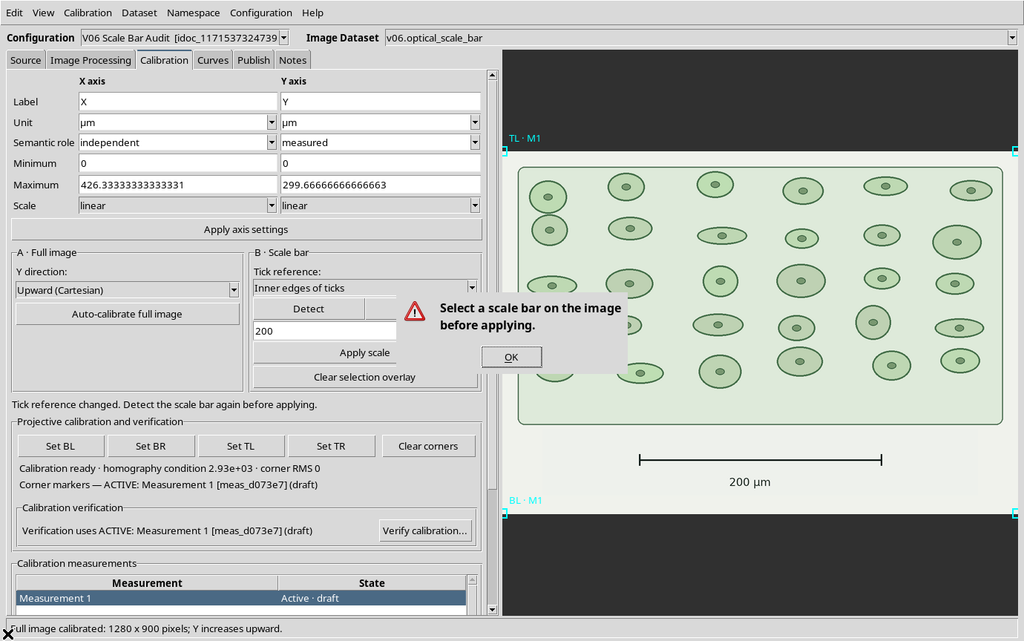
The calibration previously applied remained intact in the CORE, while the selection preference changed to inner. Changing the choice does not cause a silent recalibration.
9. Inner Ticks: 597 Pixels
Select Inner edges of ticks, press Detect and click on the bar stroke again. In our fixture, the detector found a distance of 597 source pixels.
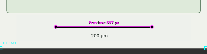
Applying 200 µm, the CORE recorded edge_convention = inner, method = detected, pixel_length = 597. The factor is 200 / 597 ≈ 0.335008375 µm/px; the axis maxima become about 428.475712 µm (X) and 301.172529 µm (Y).
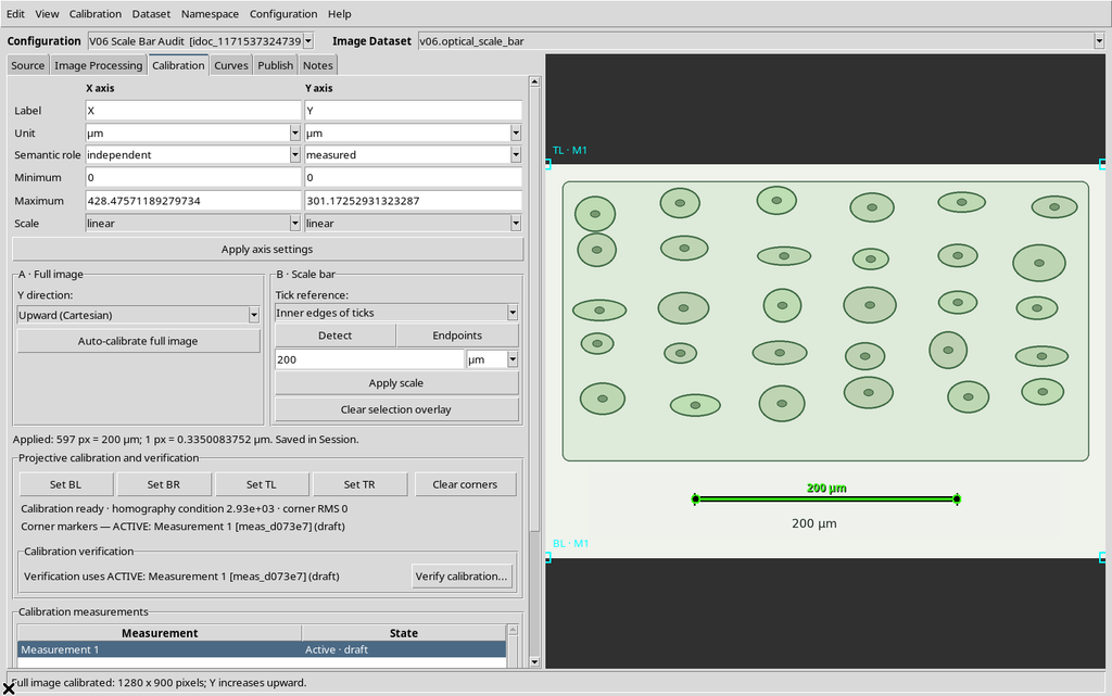
The difference from the center is due to the width of the ticks, not to new pixels added to the image.
10. Outer Ticks: 603 Pixels
With Outer edges of ticks, the detected proposal measures 603 source pixels.
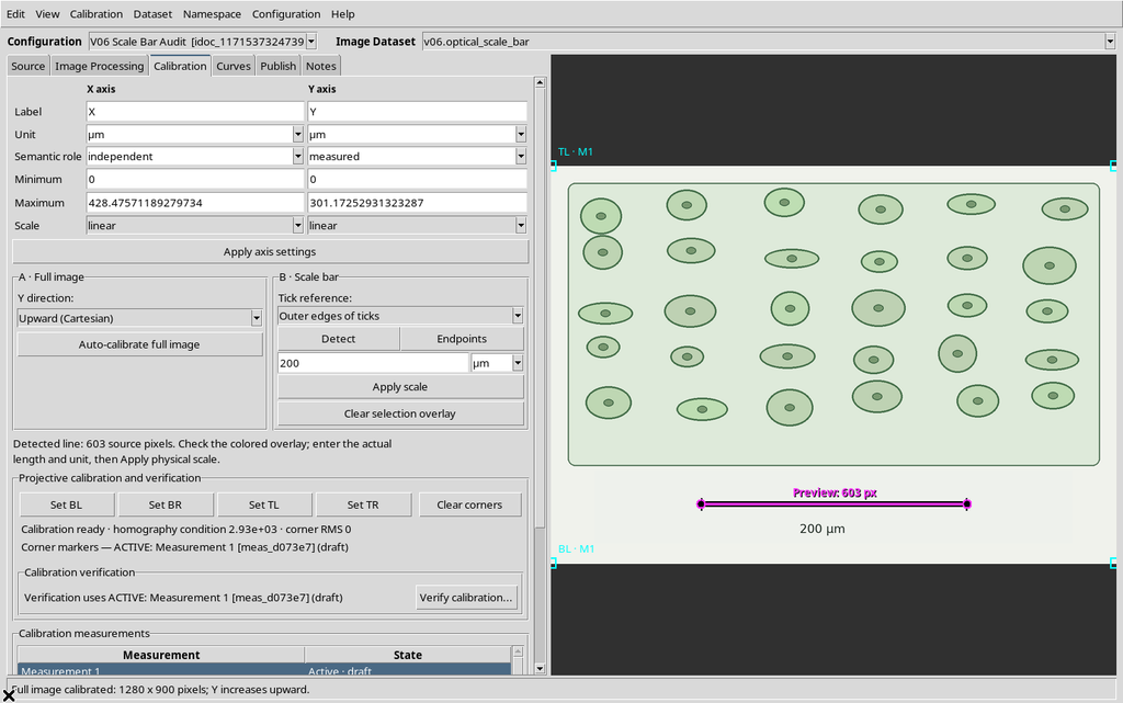
After Apply scale with the same length of 200 µm, the factor becomes 200 / 603 ≈ 0.331674959 µm/px, with maxima of about 424.212272 µm (X) and 298.175788 µm (Y).
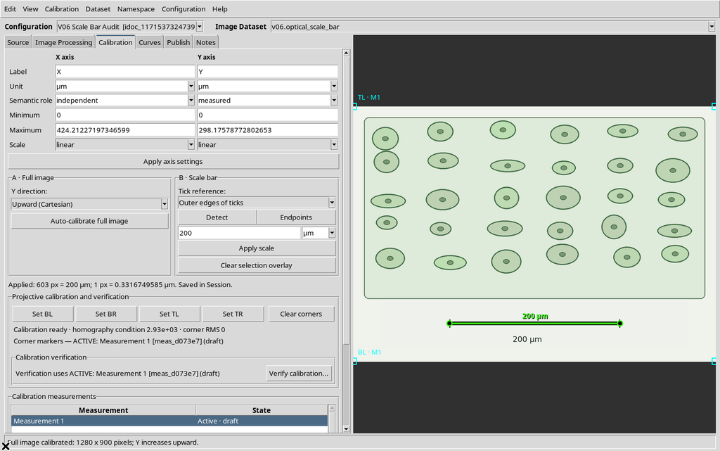
The three distances of 597, 600 and 603 px are not replicate measurements of the same definition: they use different conventions. For an experimental image you must consult the documentation of the source, not choose the convention that produces the preferred figure.
11. Manual Selection with Endpoints
When Detect does not work or the proposal is not adequate, choose Endpoints. Click the first endpoint on the raster: a temporary marker appears along with the text First endpoint selected. Click the opposite end of the bar.
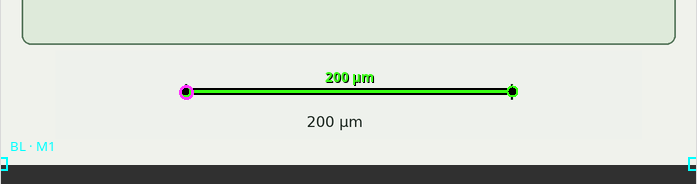
A second click too close to the first was rejected with Select two distinct endpoints, at least 3 pixels apart.
A subsequent click on the other end produced a magenta manual proposal, 598.5611511 source pixels long.
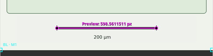
The difference of about 1.44 px from the 600 px center detection comes from clicking on integer canvas coordinates and from the inverse transformation to source pixels. It must not be hidden artificially: the manual method keeps the actual selected points.
12. Manual Application in Nanometers
The manual proposal was applied by declaring 200000 nm, a physical length equivalent to 200 µm.
The Viewer saved method = manual, edge_convention = center, pixel_length = 598.561151079, physical_length = 200000, unit = nm. The resulting factor is 334.1346154 nm/px.
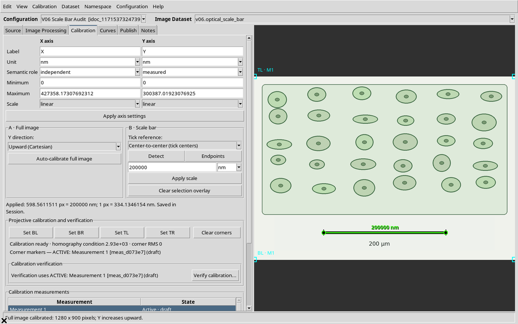
The Workspace reported the axes in nm, with maxima of about 427358.173 nm (X) and 300387.019 nm (Y). The physical unit changed, but the manually chosen pixel distance is also slightly different from the automatic proposal: therefore the numerical results are not identical after unit conversion.
13. Reset physical scale...: Two Confirmations Observed
The Calibration → Reset physical scale… command first asks:
Reset the physical scale to full-image pixels? Original raster points remain unchanged.
The No choice was exercised, verifying that the Workspace kept the manual scale and the nm unit.
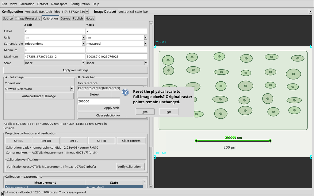
Then choosing Yes, the viewer opens a second confirmation:
Replace the existing calibration and axis limits with full-image pixel coordinates? Existing digitized points will be recalculated, not deleted.
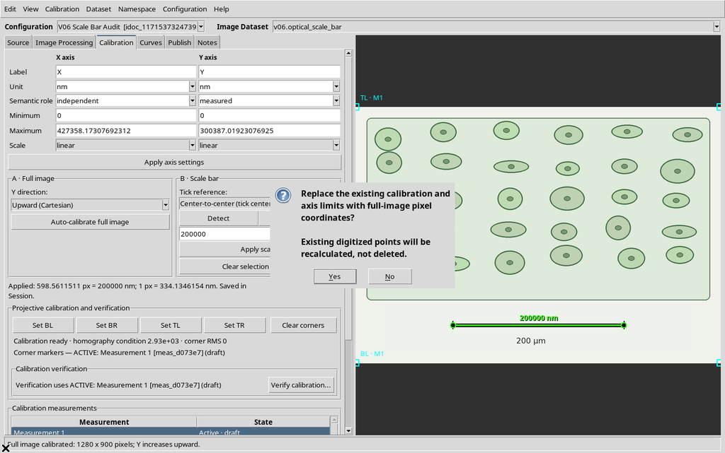
The second Yes was exercised as well.
14. Returning to Pixel Axes
After the double confirmation, the Workspace returned scale_reference = null, X axis 0–1279 px, Y axis 0–899 px, and the four corners of the full-image calibration still present.
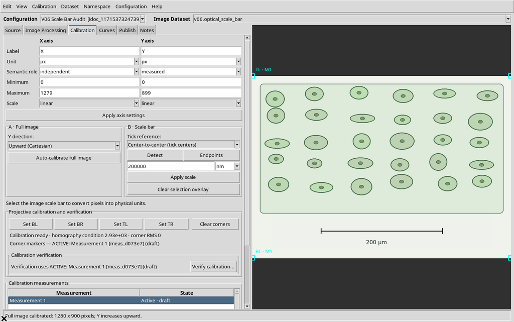
The original image and its SHA-256 remained unchanged.
15. Final Restore and Reopening the Viewer
After the reset, to leave a usable configuration, the automatic measurement Center-to-center, 600 px = 200 µm was repeated, followed by Apply scale.
The Viewer was closed through the normal window protocol and reopened from the Digitalizer entry of the Viewers catalog. The Workspace kept the same source, the calibration, the detected method, the center convention, the axes in µm and the physical length. The green overlay with the 200 µm label reappeared in the interface.
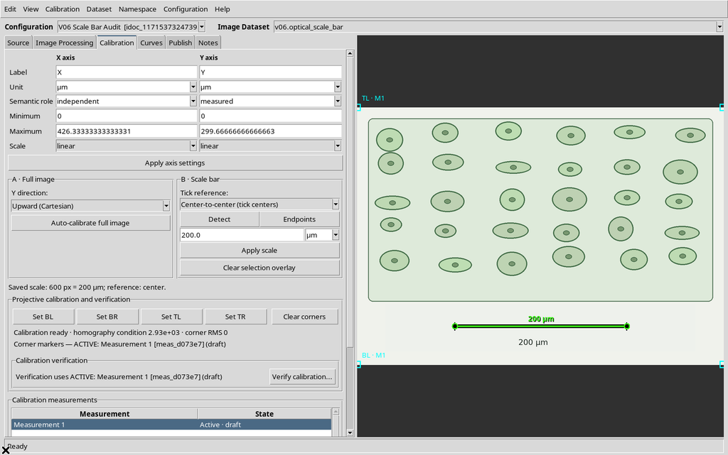
This is a restore within the same Session. It does not guarantee survival of a crash, a Session change or an image replacement, topics reserved for V27–V28.
16. Meaning and Scientific Limits of the Factor
The program measures the Euclidean distance between endpoints in source pixels, then assumes an isotropic scale over the whole image. It does not correct perspective, optical distortion, non-square pixels or a wrong label in the original image.
The detection code uses the local contrast of the bar and the geometry of the two ticks. The center/inner/outer criterion depends on the convention of the source, not on a universal property of every micrograph.
The precision of the computed digits is not an estimate of metrological uncertainty. Errors in the real length of the bar and in the location of the endpoints were not quantified in V06; uncertainty propagation and covariance require the dedicated guides and public APIs.