

Smoothness and Exclusion Paths
Assisted digitizing is not simply a matter of finding the darkest line in a figure: you have to choose the path consistent with the phenomenon studied, especially when the raster contains other curves, grids or overlapping marks. The GX-TXT Curve Digitalizer provides two complementary tools: Smooth curve prior, which affects the regularity sought, and Exclusion paths (red X), which penalize competing regions. This guide shows how to use, compare and save them without confusing temporary proposals with accepted numerical points.
1. Source and Prerequisites
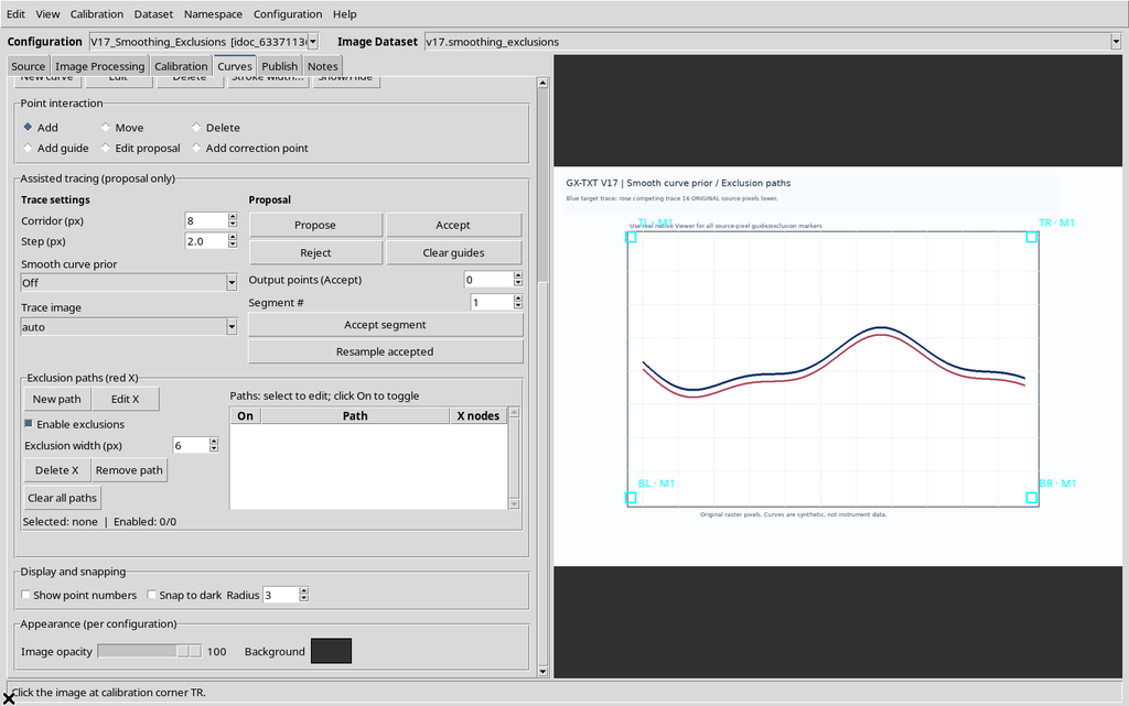
You start from an Image Dataset already loaded, with a valid axis calibration and at least one series in the Curves tab. In the example, a synthetic 1280 × 900 pixel figure contains a blue curve to follow and a nearby pink curve: the two traces are about 16 original pixels apart vertically.
The calibration assigns X from 0 to 10 s and Y from −20 to 80 mV. The target series Blue target initially has zero points: none of the tests in this guide needs Accept.
2. Where Smooth Curve Prior Is
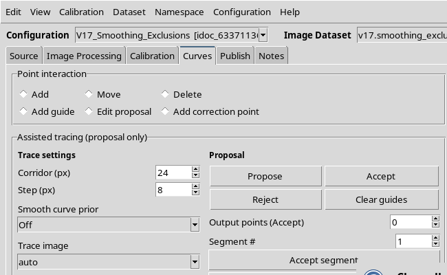
In Curves → Assisted tracing (proposal only), the Trace settings frame contains Corridor (px), Step (px), Smooth curve prior and Trace image. The Smooth curve prior field lets you select Off, Gentle or Strong.
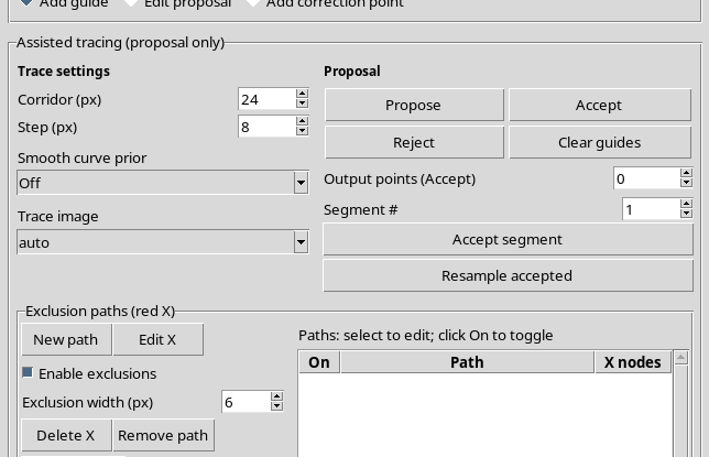
The smoothing preference acts during the search for the trajectory. It is not a filter applied after acquisition, it does not alter the source raster and on its own it does not turn a proposal into scientific points.
3. Preparing Guides and Constant Parameters
To compare the three modes, five orange guides are placed on the blue line. In the example Step = 8 px, Corridor = 24 px and the same original image are kept, with no processed version. The five guides delimit four candidate segments.
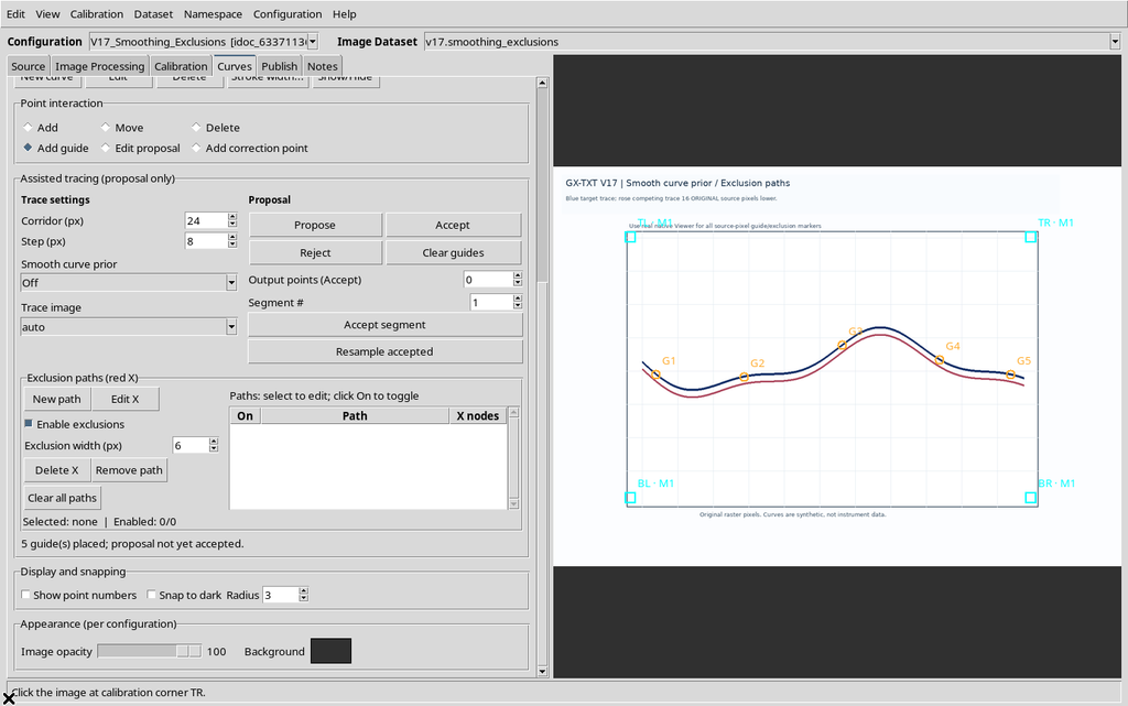
Every guide is a reference geometrically imposed by the operator: it is not automatically an accepted measurement. Keeping guides, Corridor and Step constant makes it possible to attribute any differences to Smoothness alone.
4. Generating the First Proposal with Off
Select Off and press Propose. The Viewer draws the cyan candidate and shows a summary with the mode, Step, number of points and segments.
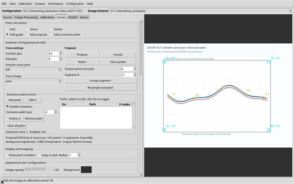
With these five guides the result is 105 provisional points over four segments. The path must be inspected on the raster to tell the blue curve apart from the competing pink trace.
5. Selecting Gentle
Change Smooth curve prior to Gentle. If there is an unaccepted proposal and the guides are still valid, the Viewer automatically starts generating a new candidate.
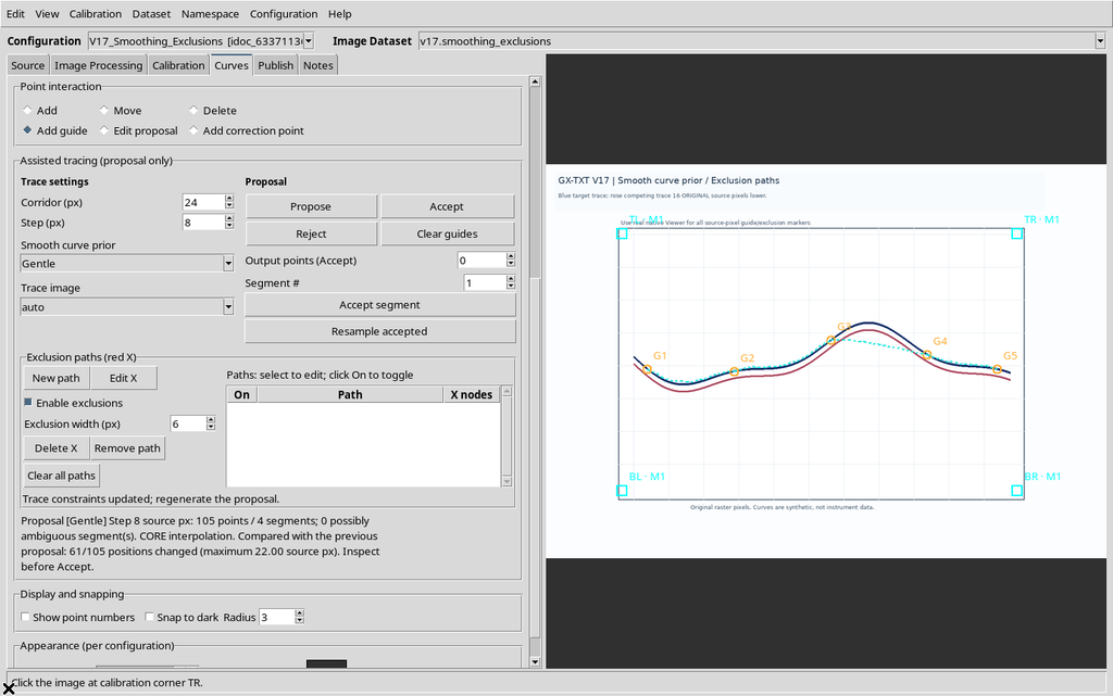
In the comparison shown, Gentle changes 61 positions out of 105 compared with Off, with a maximum shift of 22 source pixels. The five guides stay fixed. The choice neither produces nor deletes accepted numerical points.
6. Selecting Strong
Switch to Strong to favor smoother changes of direction more strongly within the search cost.
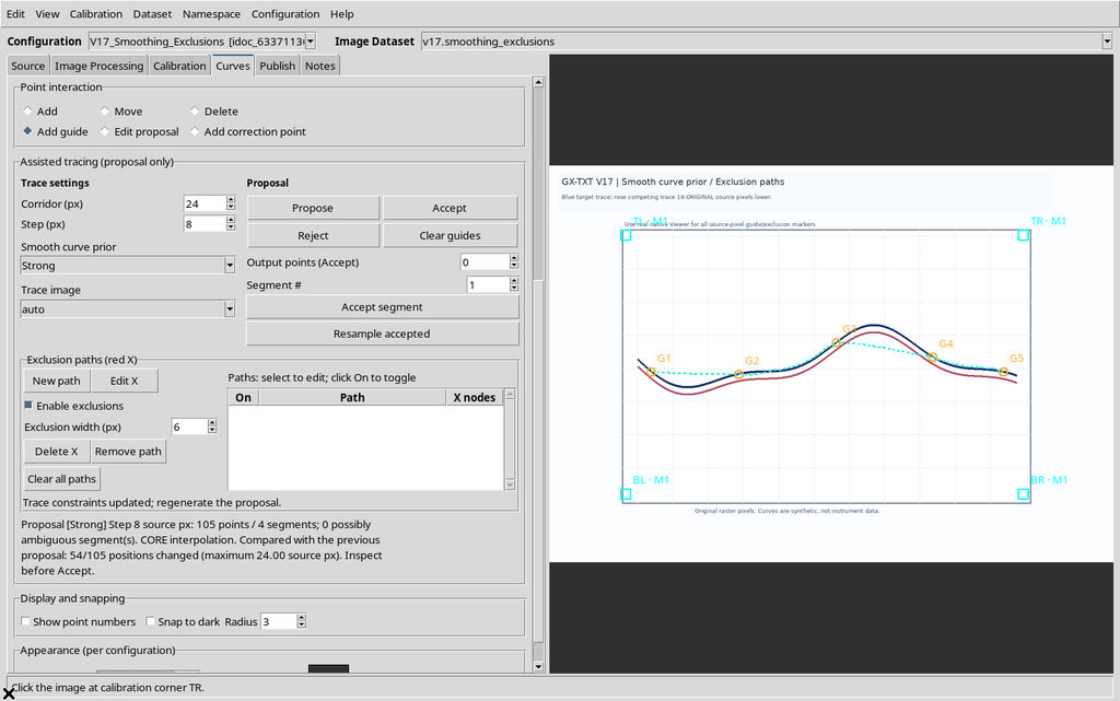
Compared with the Gentle proposal, 54 positions out of 105 change, with a maximum shift of 24 original pixels. The candidate line can still have curvature and changes of concavity: Strong does not mean replacing it with a polynomial or imposing a mathematically monotonic shape.
7. Going Back to Off and Checking Reproducibility
Setting the field back to Off, the Viewer regenerates the proposal. Under the fixed conditions of the test, the resulting trajectory coincides, vertex by vertex, with the first Off candidate.
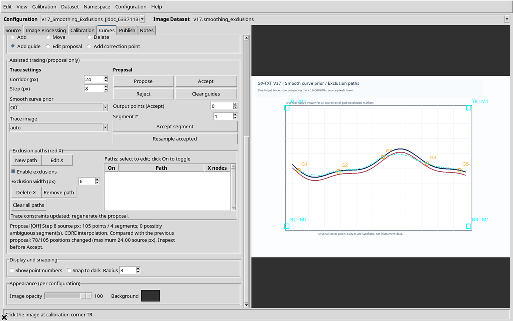
This check is more informative than a simple visual comparison: it avoids attributing to the Smoothness parameter differences actually due to a moved guide or a new image.
8. Geometric Comparison of the Three Modes
The synthetic blue curve has a known reference trajectory in original pixel coordinates:
y_px(x) = 440 + 58 sin(2π(x−200)/720) + 20 sin(2π(x−200)/305)
The positions of the vertices drawn by the Viewer can be compared with this function. For the test with Step 8 and Corridor 24 the result is:
| Smooth curve prior | Proposed points | Segments | Mean absolute vertical deviation | Vertical RMSE |
|---|---|---|---|---|
| Off | 105 | 4 | 7.94 px | 10.55 px |
| Gentle | 105 | 4 | 10.42 px | 16.43 px |
| Strong | 105 | 4 | 13.85 px | 19.83 px |
Here Off follows the synthetic reference best. This does not mean that Off is universally better: with noise or smooth contours the other modes may be more appropriate. The deviations in pixels are geometric diagnostics against a known synthetic curve, not metrological uncertainties or confidence probabilities.
9. When Smoothness Can Be Counterproductive
Too strong a regularity constraint can flatten narrow peaks, sharp corners or real abrupt changes. If the phenomenon has a significant discontinuity, start from Off and increase the regularity only when the raster justifies it.
The proposal must be inspected before any acceptance: a path that looks smoother is not necessarily more faithful to the experimental data.
10. What Exclusion Paths Are
Below the tracing commands is Exclusion paths (red X). The operator can draw one or more paths with red X crosses, connected by a spline. The surrounding region adds a soft exclusion cost to the search.
Unlike a mask, this cost does not absolutely forbid crossing a region. The real line can correctly cross another curve: deciding to exclude therefore requires a scientific judgment.
11. Creating a Path with New Path
Press New path after selecting the target curve. A row appears in the path table, initially with zero nodes. The Viewer switches to the mode that lets you place X marks on the raster.
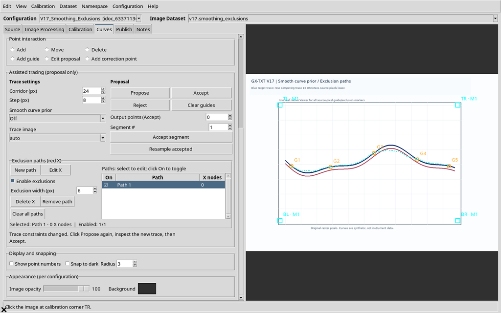
An empty row can be enabled, but a geometric exclusion requires at least two nodes. Enabling it does not change the table of accepted points.
12. Placing the First X Nodes
Click on the trace you want to discourage. Each click adds a red cross on the Canvas in original image coordinates.
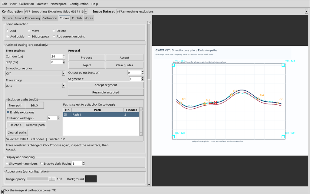
The red X marks must not be confused with the orange G guides: the guides constrain the path being sought; the X marks indicate regions whose crossing should become less favorable.
13. Building the Exclusion Spline
Continuing with more clicks gives a continuous path. In the example Path 1 contains seven X nodes, spread over the central region of the blue line.
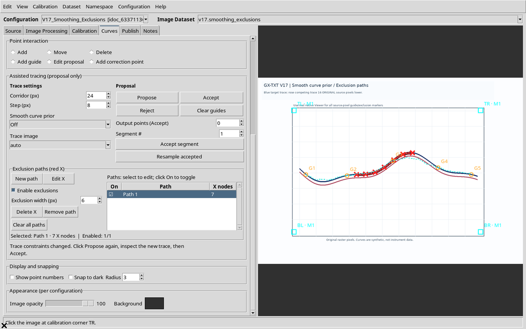
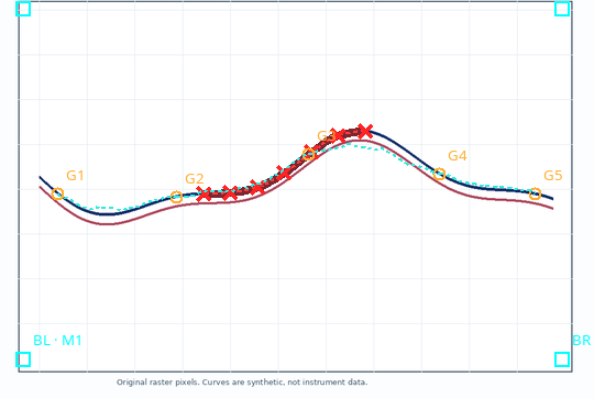
Here the choice is deliberately wrong: we are excluding the curve we know to be correct, to show in a controlled way the consequences of an inappropriate constraint.
14. Recomputing After Changing the Exclusions
When X marks are added or changed, the previous proposal is considered out of date. The Viewer requires you to repeat Propose and check the new trajectory. Changing a spline is not the same as already having a new valid result.
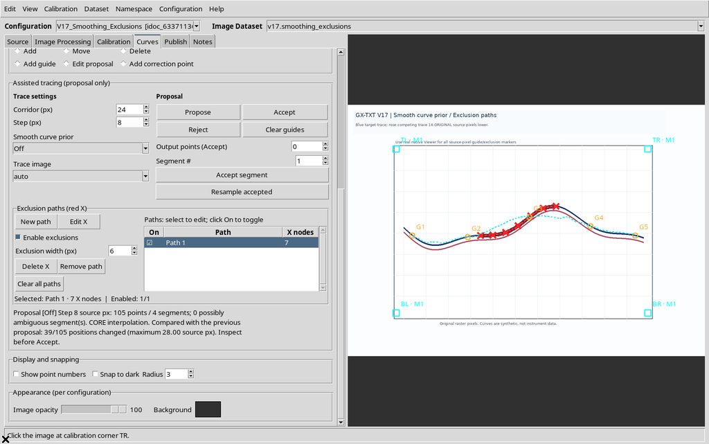
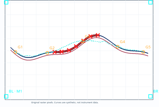
The candidate line is recomputed taking the exclusion cost into account, while still respecting the constraints of the orange references. A candidate generated before the change must not be attributed to the new exclusion.
15. A Wrong Exclusion Can Make the Tracing Worse
With Smoothness Off, Step 8 and Corridor 24, introducing Path 1 on the blue line changes 39 vertices out of 105, with a maximum shift of 28 original pixels.
| Search configuration | Mean vertical deviation from the blue curve |
|---|---|
| No exclusion | 7.94 px |
| Path 1 active, Width 6 px | 13.62 px |
| Path 1 active, Width 18 px | 15.79 px |
| Path 1 and Path 2 active, Width 18 px | 15.87 px |
The result shows why it is not enough to identify a dark area: a red path placed on the right trace penalizes it, possibly moving the candidate onto other marks in the image. These figures are only geometric comparisons on a synthetic raster.
16. Disabling a Single Path with the On Column
In the exclusion table, a click on the On cell of the selected path enables or disables it. The symbol switches between checked and unchecked, and the drawing is dimmed when the path is disabled.
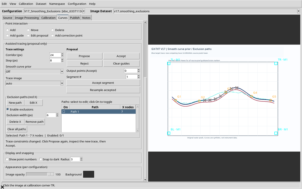
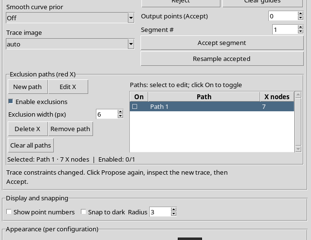
Selecting the row serves to choose which path to edit: it is not the same as enabling it. A disabled path keeps its nodes and can be re-enabled without rebuilding them.
17. Checking the Effect of Individual Enabling
After Path 1 is disabled, a new Propose returns exactly to the trajectory obtained without exclusions.
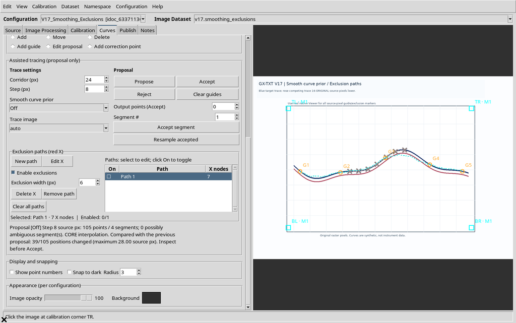
Re-enabling Path 1 and repeating Propose reproduces the candidate with exclusion. This comparison separates the mere visibility of the markers from their actual participation in the calculation.
18. Enable Exclusions: The Global Command
The Enable exclusions control disables or re-enables all the exclusion penalties of the curve, without deleting the paths and without changing the individual On checkboxes.
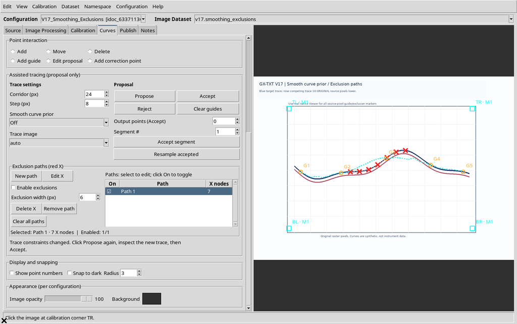
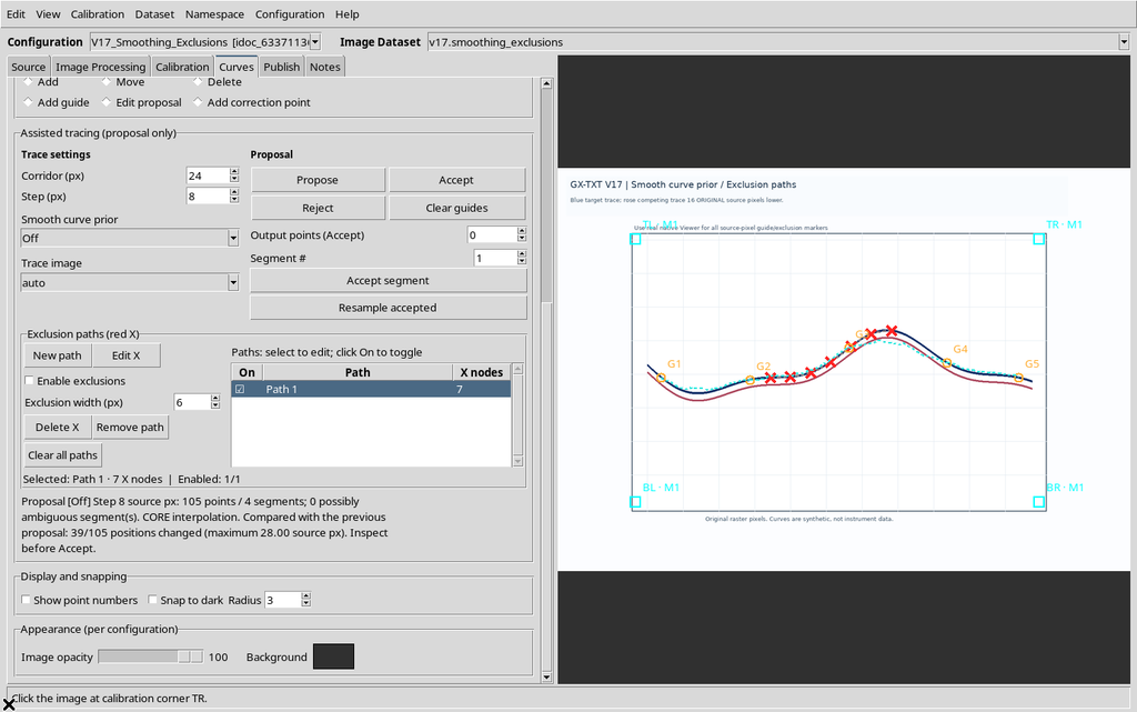
In our example the proposal with exclusions globally off coincides with the initial one without exclusions. The command is particularly useful to compare two candidates while keeping the drawn splines identical.
19. What Exclusion Width (px) Controls
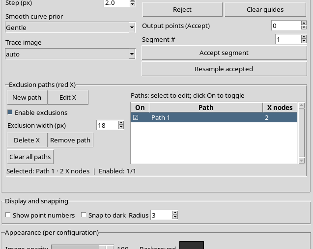
Exclusion width (px) defines the width of the penalized corridor around the spline, in the coordinates of the original raster. It does not change the thickness of the scientific curve, the Corridor value of the proposal or the physical scale of the axes.
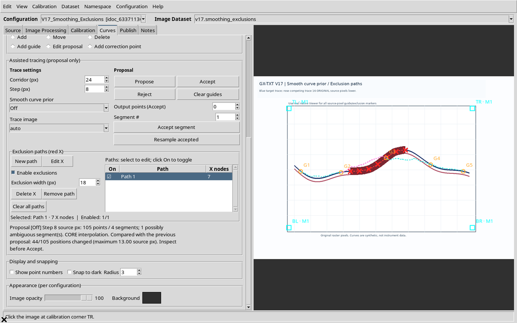
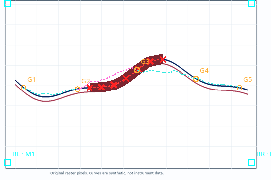
Going from Width 6 to Width 18, with Path 1 active, the tracing changes further: 44 positions out of 105 are different and the maximum shift between the two proposals is 13 source pixels. After every change of Width you need to press Propose to see the new result.
20. Width Limits and Normalization
In the version shown the effective width is between 1 and 40 original pixels. Entering 0, the field is automatically set back to 1.
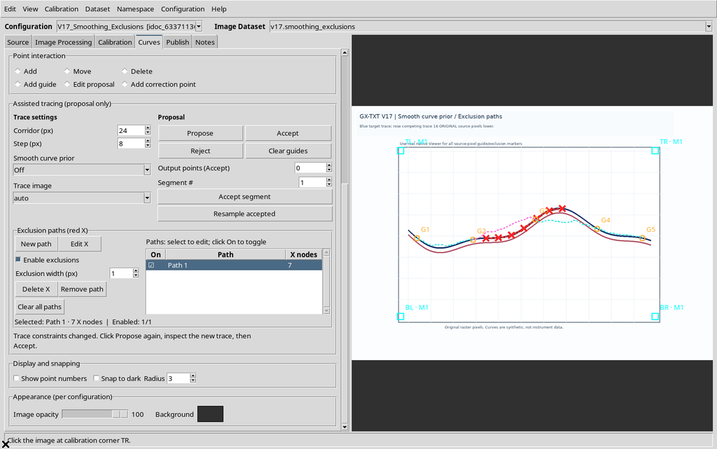
Entering 45, the field is set back to the maximum of 40.
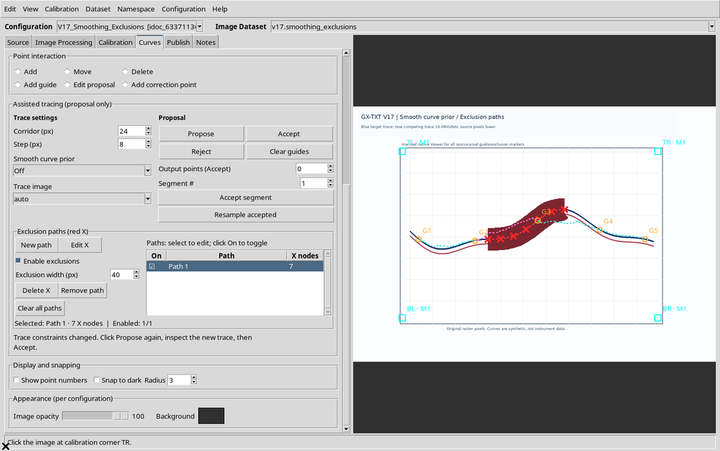
This normalization does not mean a proposal was obtained with an invalid value. Always check the number actually shown after the field is confirmed.
21. Drawing Two Independent Paths
With New path a second path can be created. The table lists Path 1 and Path 2, each with its own number of nodes and its own On switch.
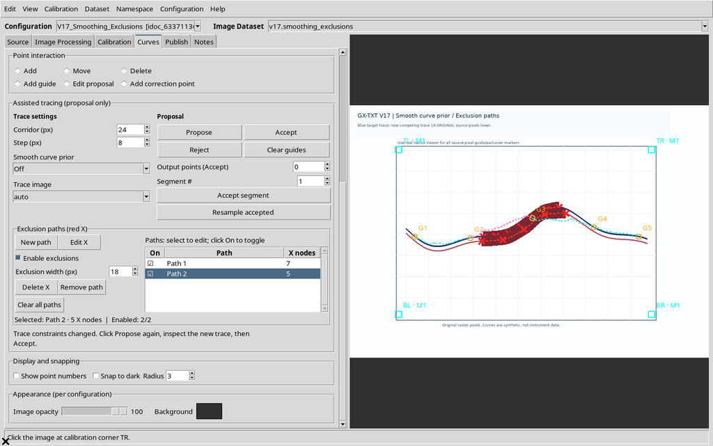
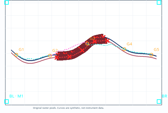
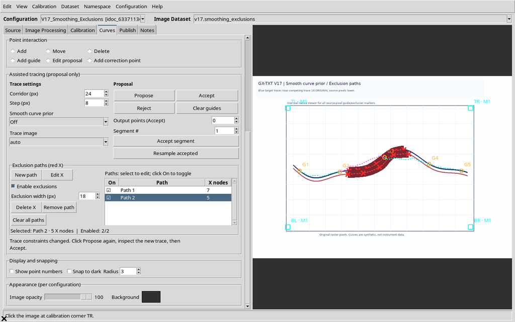
In the example, Path 1 has seven X marks on the blue line and Path 2 has five along the pink line. A spline describes the region to penalize; it is not a new numerical curve.
22. Proposal with Two Paths Enabled
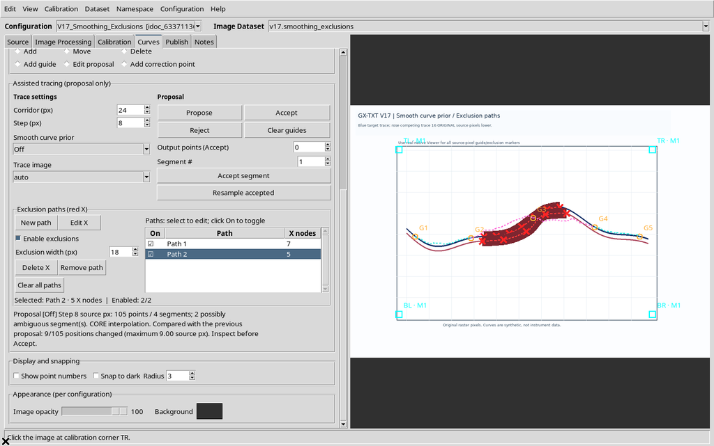
With both paths active and Width 18, Propose uses the respective penalties during the search.
Disabling only Path 2, the second spline stays visible in dimmed form.
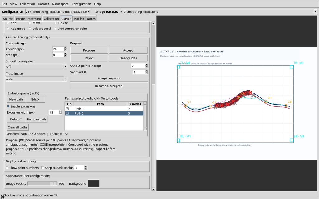
Repeating Propose with only Path 1 active gives the same geometry measured earlier for Path 1 with Width 18.
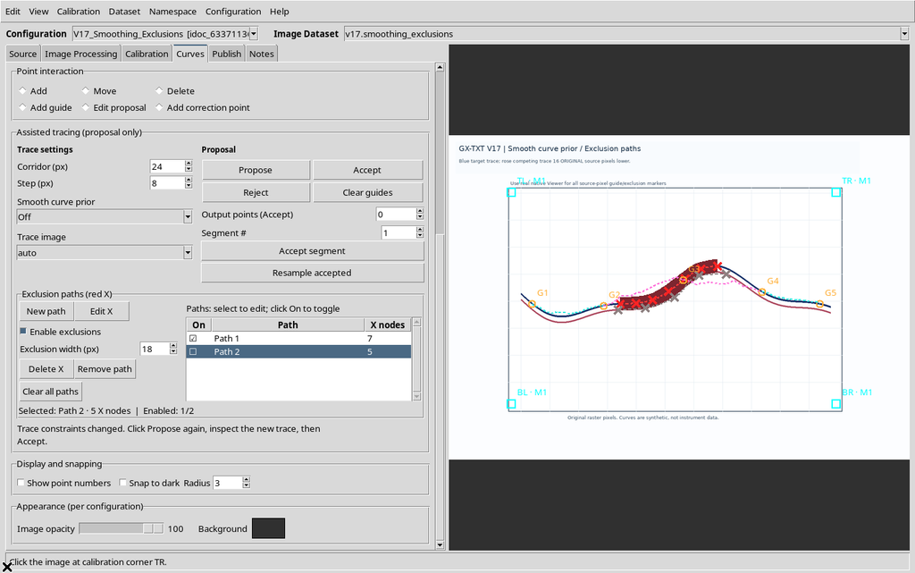
The comparison shows that the On checkboxes work independently. If two exclusions overlap or one involves the correct curve, the outcome must be checked against the original data.
23. Editing an X Node by Dragging
To correct an existing spline, select the desired path, use Edit X and drag an X to its new position. The program records the action in the configuration history.
The moved node keeps its position within the same path. Edit → Undo restores the previous coordinates, while Edit → Redo reapplies the move. A complete drag is one history change, not a sequence of micro-operations to publish.
24. Delete X and the Undo/Redo History
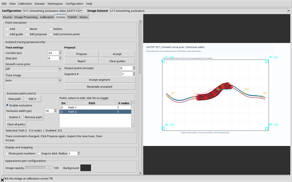
The Delete X button deletes the last node of the selected path, leaving the others intact. In the example Path 2 goes from five to four nodes.
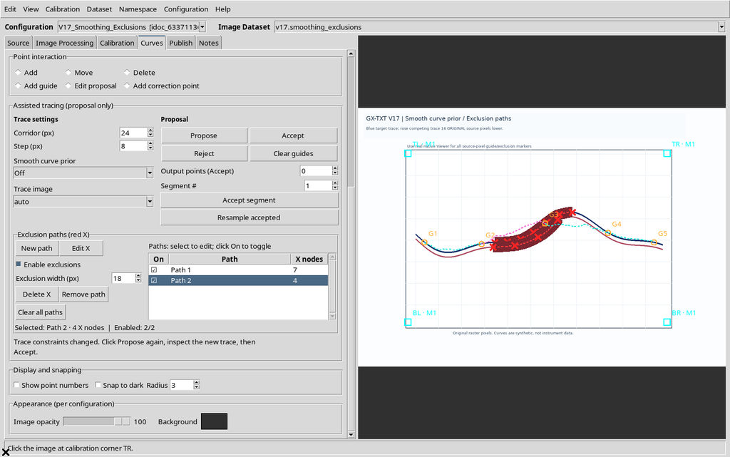
With Undo it goes back to five; with Redo back to four; another Undo restores all five again.
These commands act on the exclusion geometry, not on the scientific points of the curve. The history can also include other configuration changes, so check which action was the last one before pressing Undo.
25. Remove Path: Deleting a Whole Path
Select the desired row and press Remove path to delete the whole path, not just the last X.
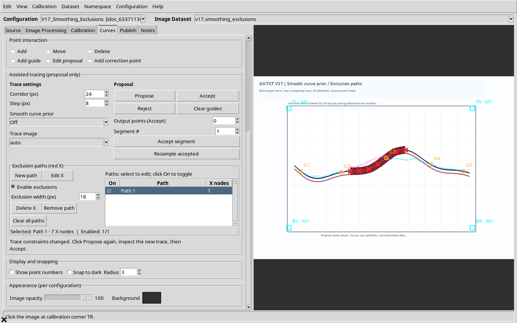
If the deletion was not wanted, Edit → Undo rebuilds the whole path with the same nodes and the same identity.
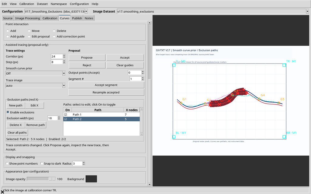
Path 1 stays separate from the operations applied to Path 2.
26. Clear All Paths and Explicit Confirmation
Clear all paths asks for confirmation before deleting the exclusion paths. The message also states that accepted points and published Datasets are not what is being deleted.
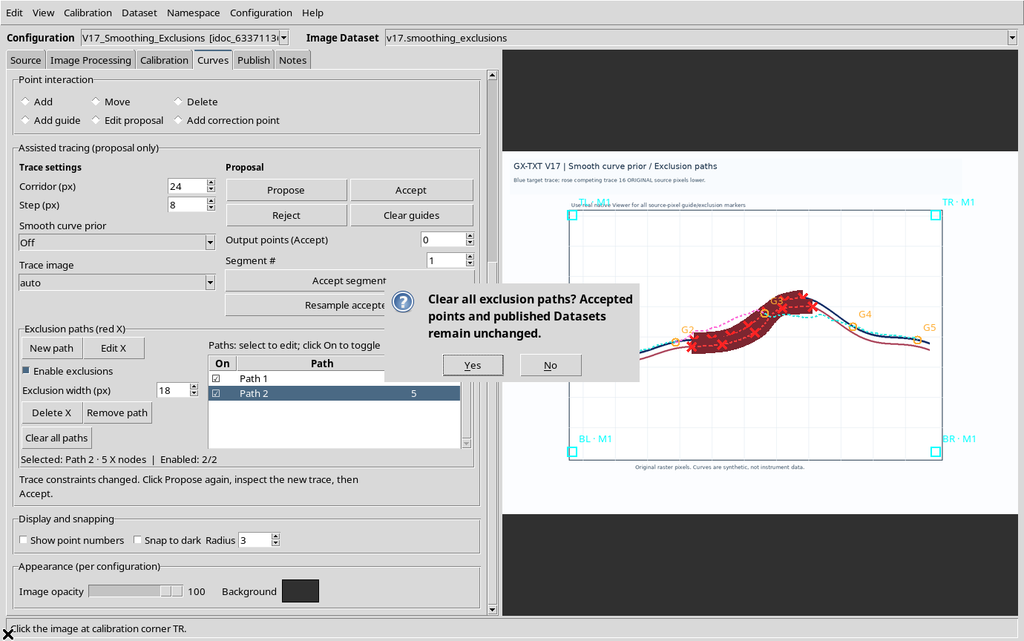
Choosing No, the paths remain available.
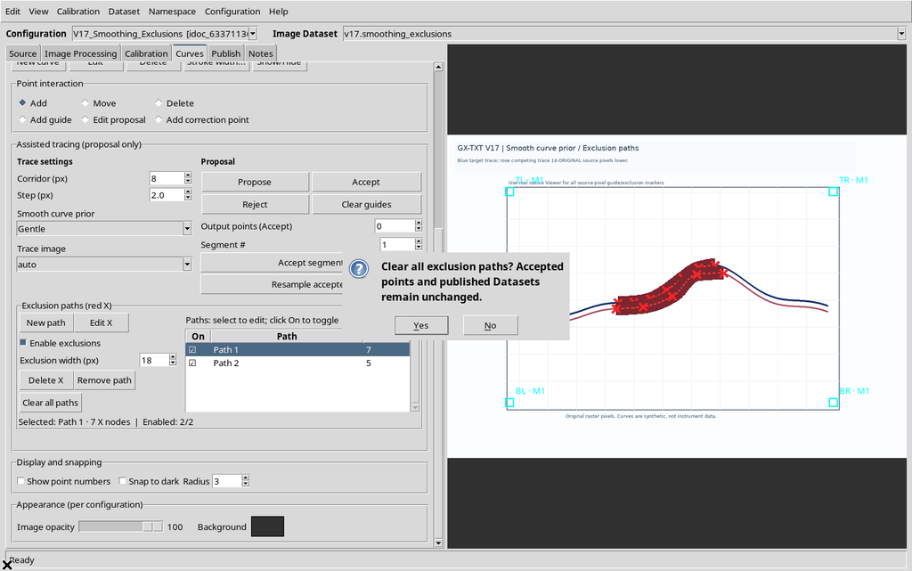
The example uses series with no accepted numerical points. The interface states that any Datasets already published are not deleted, but this case is not illustrated with a pre-existing Dataset.
27. Clear All Paths with Yes and a Subsequent Undo
Confirming Yes, the exclusion table becomes empty and the red splines disappear from the Canvas.
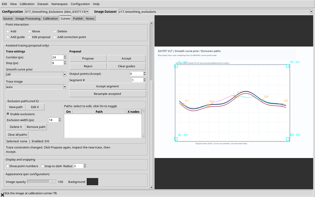
Pressing Edit → Undo, the two paths come back with their nodes and their own identifiers.
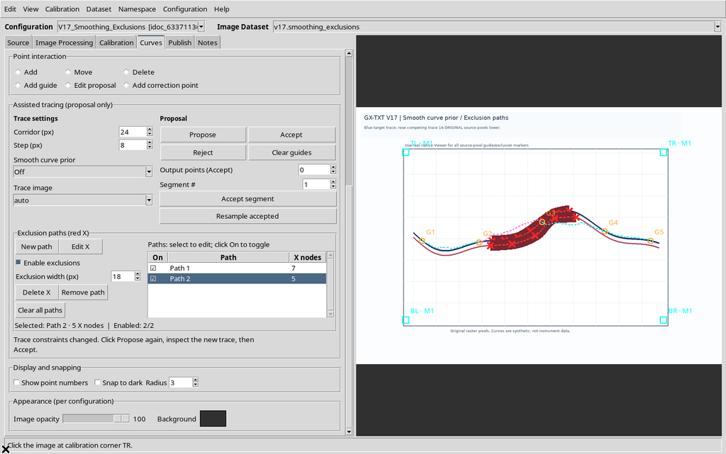
This recovery option does not replace regularly saving the configuration.
28. Exclusion Paths Belong to the Selected Curve
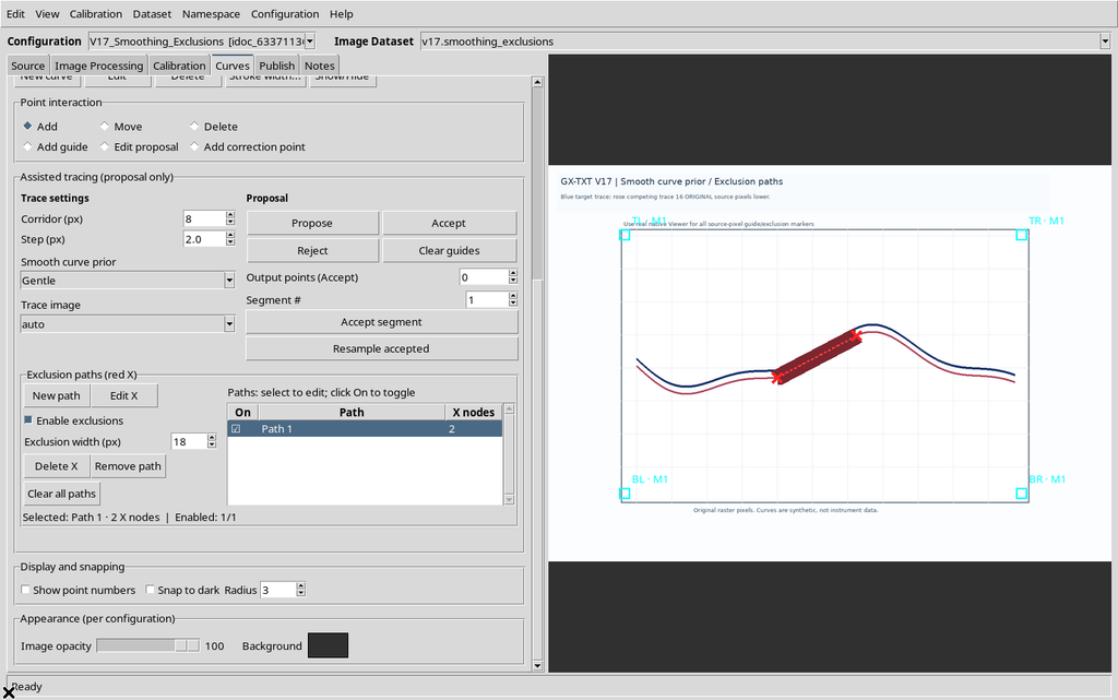
To check the scope of the paths, we create a second, empty numerical series, Control curve. When it is selected, the exclusion table is initially empty.
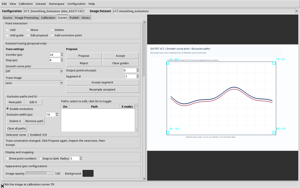
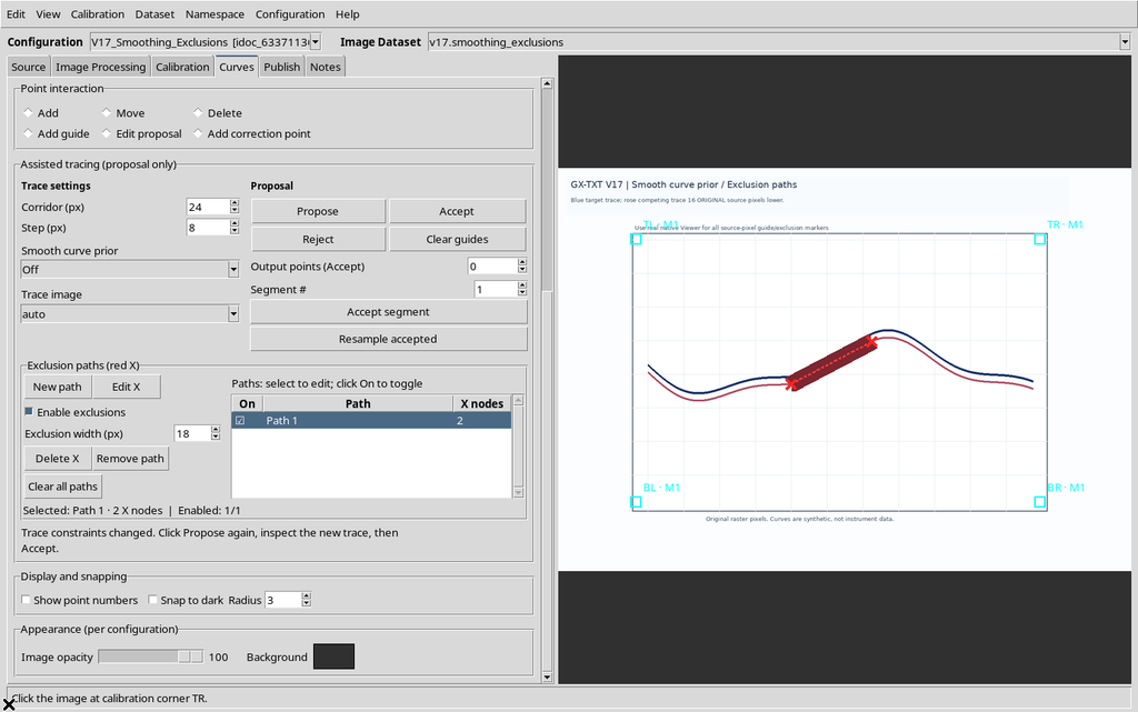
We add a path of its own with two X nodes to this series.
Going back to the first series, Blue target, its two original paths of seven and five nodes appear again.
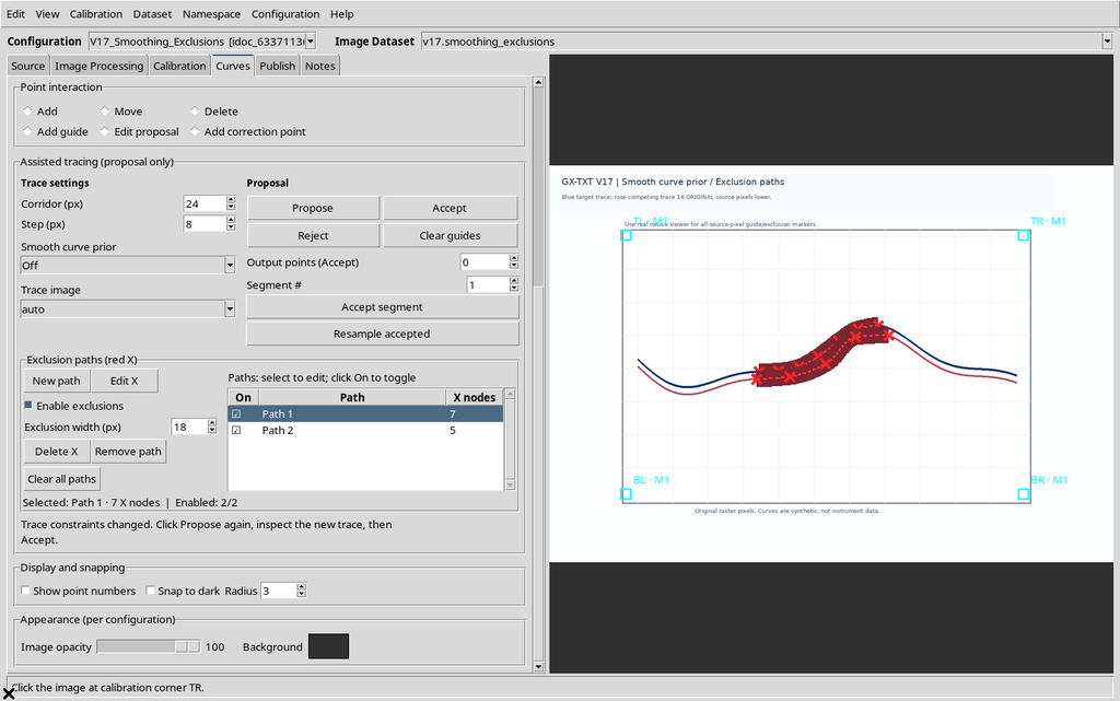
The paths are therefore associated with the individual series and with the original source, not a single undifferentiated graphic mask shared by all the curves.
29. Saving the Settings and the Paths
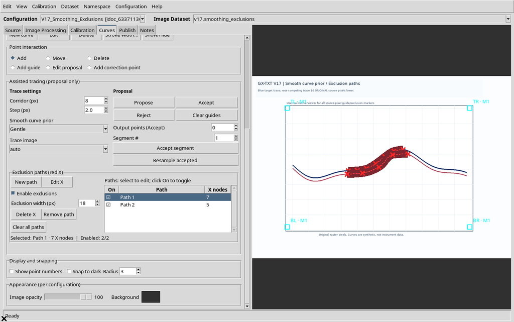
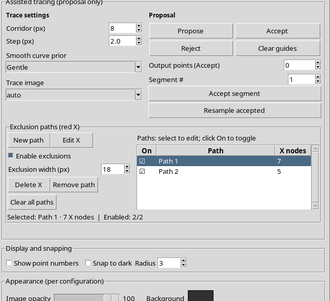
The Smooth curve prior mode, the global enabling of the exclusions, Width and the geometry of the splines belong to the current configuration. The final choice shown here is Smoothness = Gentle, Width = 18 px, with the paths still kept.
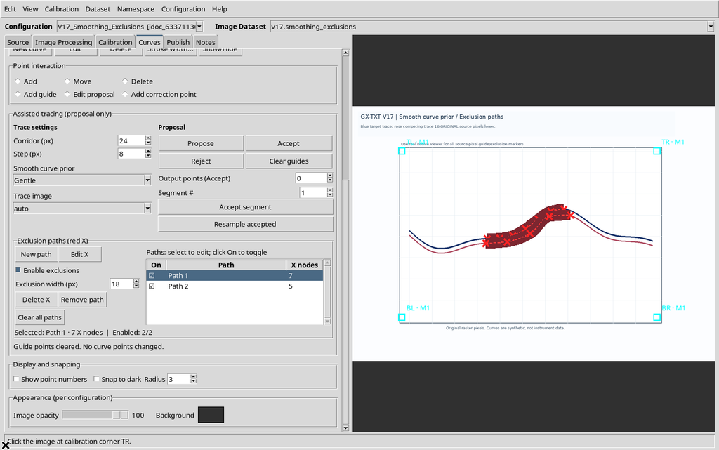
To keep them, use Configuration → Save configuration, then close the Viewer normally. The temporary proposals must not be confused with the constraints saved in the configuration.
30. Reopening the Same Session
Reopening Curve Digitalizer from the same Session, the Viewer recovers the source, the series, the calibration and the saved paths.
Selecting Control curve, its single two-node path appears.
Going back to Blue target, the two main paths reappear with their seven and five nodes respectively.
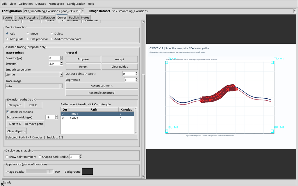
Smoothness Gentle, Width 18 and the individual enable states are kept as well. The orange guides and the current proposal, instead, are transient: they are not a scientific publication and must not be interpreted as saved points.
31. Source-Bound Constraints and Operating Limits
Exclusions are bound to the image from which they were drawn. If the configuration changes source, a spline belonging to the previous raster must not be reused automatically as a constraint for another graph.
The Viewer specifies a limit of 16 paths per curve and 200 nodes per path. A spline with fewer than two nodes does not define a continuous exclusion region.
The user must also distinguish the enabled path from the one selected in the table, and distinguish a soft penalty from an absolute prohibition of passage.
32. Suggested Operating Procedure
- Calibrate the raster and create or select the correct series.
- Place the guides consistently with the trajectory to follow.
- Try Off and, if necessary, compare it with Gentle and Strong.
- If a competing curve causes deviations, use New path and place the X nodes on the competing trace, not on the one to acquire.
- Check the selection, the On checkboxes, Enable exclusions and Exclusion width.
- Run Propose again after changing the exclusions; always compare the cyan line with the image.
- Correct any X marks with Edit X, Delete X and Undo/Redo; use Remove path and Clear all paths only when required.
- Save the configuration after checking the paths that are to be kept.
33. Scientific Summary
Smoothness regulates the cost of changing direction in the search, while Exclusion paths discourage regions drawn by the operator. The two tools are complementary and do not replace visual review. A smoother line, or one farther from the X marks, is not by definition more accurate.
In the synthetic comparison shown, Off produced the candidate geometrically closest to the blue reference. An exclusion deliberately placed on the correct curve worsened its fidelity, showing the importance of justifying every constraint. The results described are proposals to be checked: no new scientific points were accepted, no metrological errors estimated and no new numerical Datasets published.
Point-by-point review of proposals, segment acceptance and interaction with acquired points will be covered in the chapter devoted to correcting the proposal.