

Logarithmic Calibration, Mixed Axes and Y Direction
This guide (V08) documents three aspects of Curve Digitalizer: X-log/Y-linear axes, X-log/Y-log axes and the vertical direction of the full-image calibration.
1. Three Canonical Images and Three Configurations
Three reproducible synthetic images were created and imported through the GX-TXT Acquisition Handler as true Image Datasets with the image.raster contract. They are neither experimental photographs nor screenshots of the interface.
| Test configuration | Source and purpose |
|---|---|
V08 Mixed LogX LinearY | Graph with logarithmic X, linear Y |
V08 Both Axes Log | Graph with both X/Y logarithmic |
V08 Pixel Y Direction | Pixel rows to compare Upward and Downward |
2. The First Graph: Logarithmic X and Linear Y
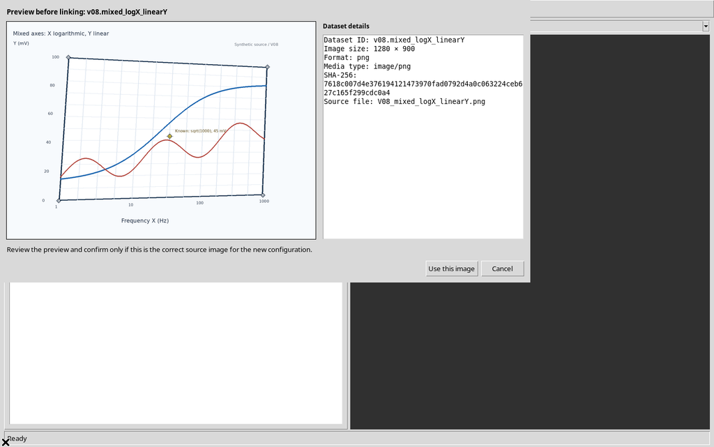
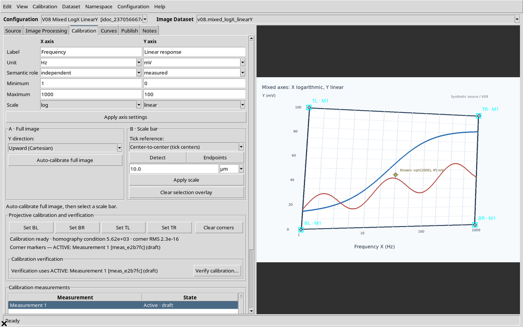
The first example shows Frequency, from 1 to 1000 Hz on a logarithmic scale, and Linear response, from 0 to 100 mV on a linear scale. The quadrilateral with four targets is deliberately in slight perspective.
After creating the Digitizer Configuration, the source was confirmed with Preview source image → Use this image. The yellow verification point nominally corresponds to about 31.622777 Hz and 45 mV.
3. Constraint: The Limits of a Log Axis Cannot Be Zero or Negative
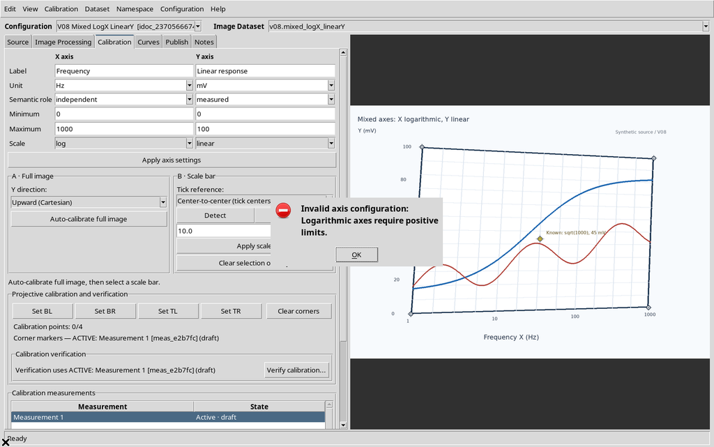
Selecting X Scale = log and Minimum = 0, the Apply axis settings command rejected the input with:
Invalid axis configuration: Logarithmic axes require positive limits.
The same check was exercised with Minimum = −1, again rejected.
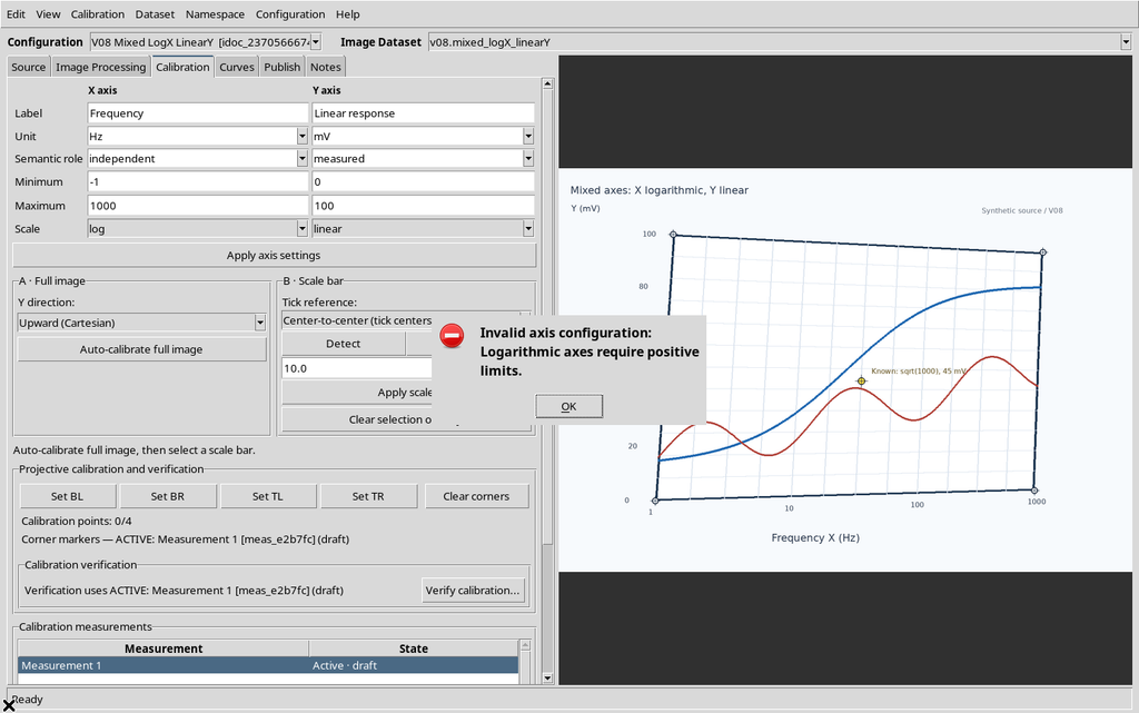
The axes of the previous Workspace remained unchanged. Both limits of every logarithmic axis must be strictly positive and different. In the mixed example, on the other hand, the limit Y=0 mV is valid, because Y remains linear.
4. Setting and Applying the Mixed Calibration
In the X axis panel, enter Label = Frequency, Unit = Hz, Minimum = 1, Maximum = 1000, Scale = log. In the Y axis panel, use Label = Linear response, Unit = mV, Minimum = 0, Maximum = 100, Scale = linear.
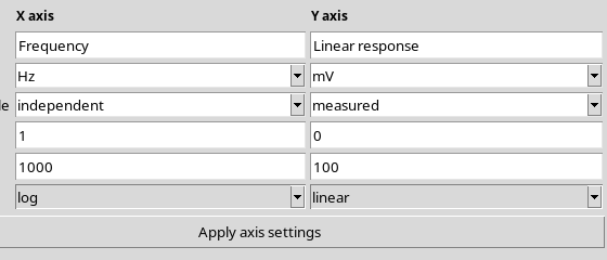
Press Apply axis settings. The framework confirms that X and Y have distinct scientific scales. These fields do not yet establish where the physical corners of the graph are in the raster.
5. Four Corners of the Mixed Source
Press the Set BL, Set BR, Set TL, Set TR buttons in order, clicking the original targets of the graph area.
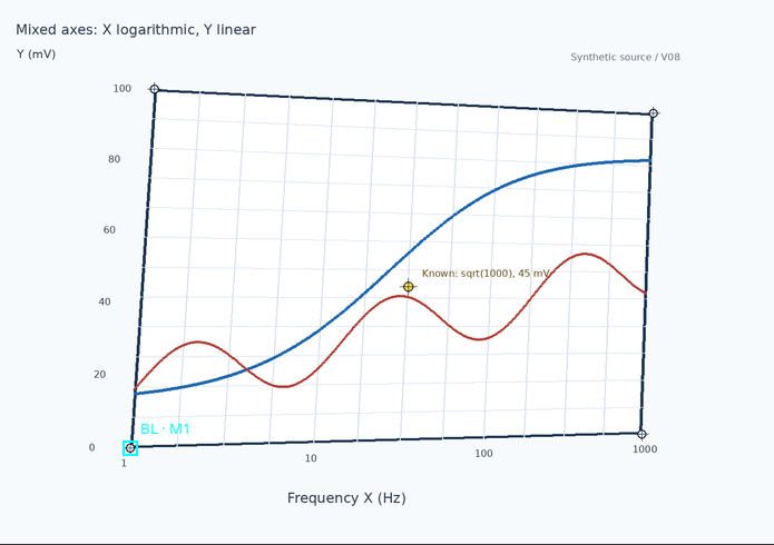
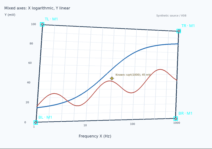
After the fourth click, the GUI showed Calibration ready, with four cyan markers. The model determined a non-affine projective homography, valid with mixed numerical axes as well.
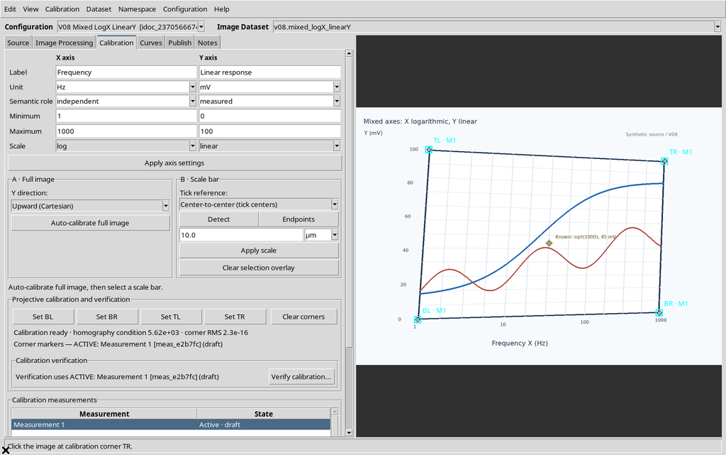
The value corner RMS ≈ 2.3×10⁻¹⁶ describes the residual of the four points used to determine the matrix; it does not measure the real uncertainty of the experiment.
6. Formula for Logarithmic X, Linear Y
After the pixels are projected into normalized coordinates (u,v), GX-TXT applies a transformation for each axis.
For logarithmic X: X = 10^(log10(Xmin) + u × [log10(Xmax) − log10(Xmin)]).
With Xmin=1 and Xmax=1000: X = 10^(3u) Hz.
For linear Y: Y = Ymin + v × (Ymax − Ymin) = 100v mV.
The synthetic control point was drawn at (u,v)=(0.5; 0.45), so its nominal coordinates are √1000 ≈ 31.622777 Hz and 45 mV. The logarithmic transformation is not a canvas zoom: it changes the scientific mapping of the coordinates.
7. Independent Verification of the Mixed Graph
With Verify calibration… open, the yellow marker was clicked in the GUI and Expected X = 31.622776601683793, Expected Y = 45 were entered. The actual Tk event (366,394) corresponded to about (674.0719; 473.0216) source pixels.
| Quantity | Expected | Calculated | Δ physical |
|---|---|---|---|
| Frequency X | 31.622777 Hz | 31.31893 Hz | −0.3038503 Hz |
| Linear response Y | 45 mV | 45.18386 mV | +0.1838589 mV |
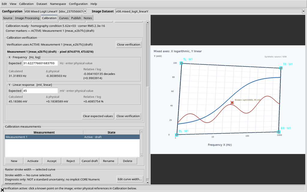
A second numerical solution of the matrix, run on the four saved corners, returned 31.3189263 Hz and 45.1838589 mV, consistent with the figures shown in the interface.
8. Decades and Percentages Are Different Comparisons
In the Relative / log column, the Viewer showed for logarithmic X:
−0.004193135 decades (×0.9903914)
For linear Y:
+0.4085754 %
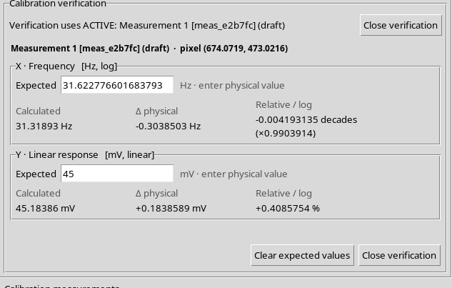
The logarithmic comparison uses log10(Calculated / Expected), while a linear relative comparison uses (Calculated − Expected) / Expected × 100%, when the reference allows it.
These numbers are residuals of a verified point, not statistical uncertainties or estimates of general accuracy.
9. Opening a Log-Log Dataset Without Relinking the First Configuration
The second example uses a new Digitizer Configuration and another source: v08.loglog_positive. The first configuration stays linked to its own Image Dataset.
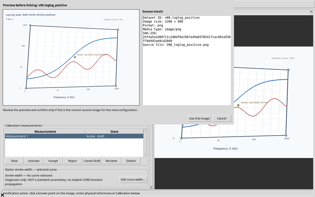
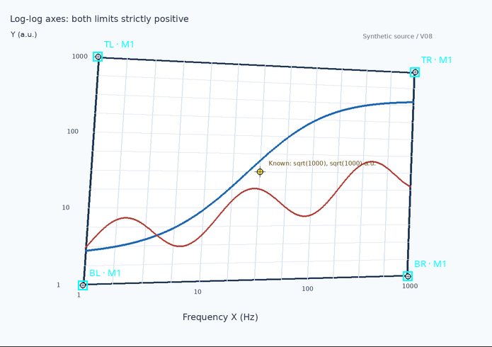
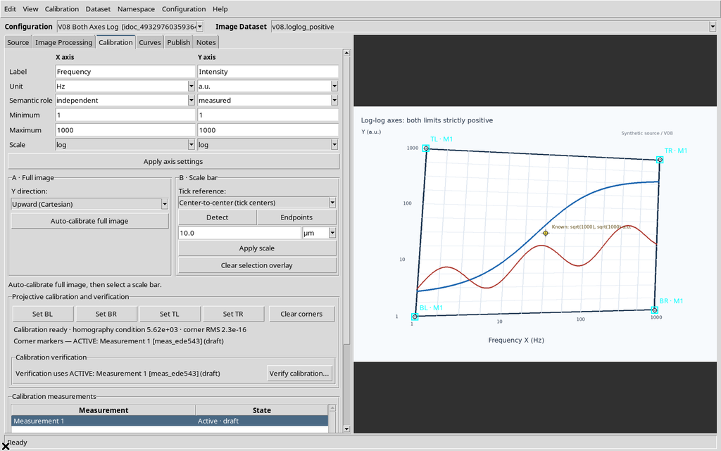
The log-log figure declares Frequency X = 1–1000 Hz and Intensity Y = 1–1000 a.u., both logarithmic. The central yellow point nominally represents √1000 on each axis.
10. Rejection of Zero and Negative Values on a Logarithmic Y
With Y Scale = log, a Y Minimum equal to 0 was tried.
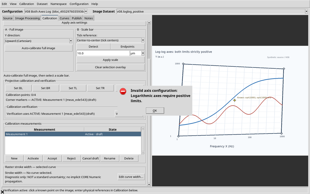
A Y Minimum equal to −1 was then tried.
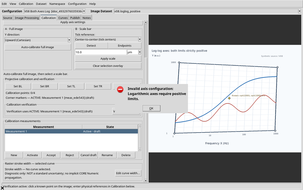
Both attempts were rejected with Logarithmic axes require positive limits.
11. Applying Two Logarithmic Axes
Fill in X Frequency / Hz, Minimum 1, Maximum 1000, Scale log, and Y Intensity / a.u., Minimum 1, Maximum 1000, Scale log. Apply through Apply axis settings.
Then acquire the four corners with Set BL / BR / TL / TR. The result is a valid quadrilateral with a single four-corner homography: the two scientific axes transform the normalized coordinates independently.
12. Mathematics and Verification of the Log-Log Graph
With both axes between 1 and 1000 on a logarithmic scale:
X = 10^(3u) Hz and Y = 10^(3v) a.u..
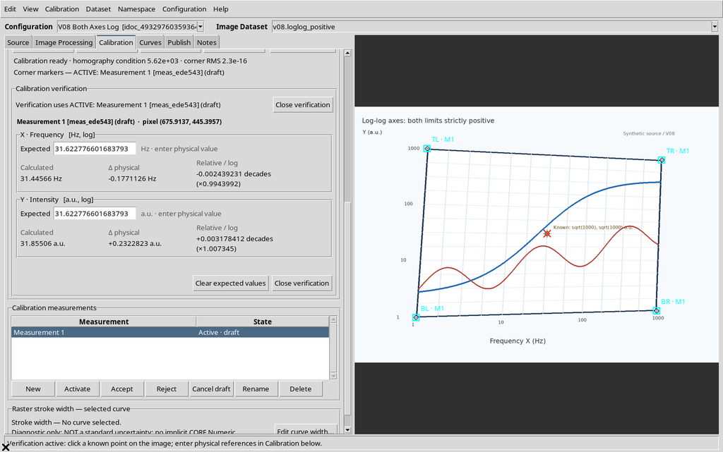
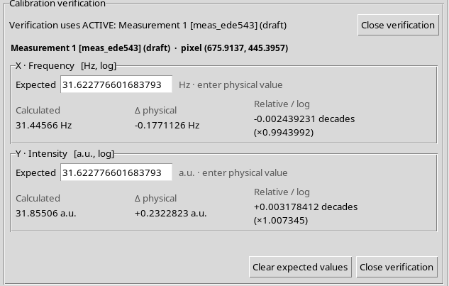
At the normalized point (0.5; 0.5), both are equal to √1000 ≈ 31.6227766. The actual click on the yellow control happened on the canvas at (367,379), equivalent to about (675.9137; 445.3957) source pixels.
The GUI showed:
| Axis | Expected | Calculated | Logarithmic residual |
|---|---|---|---|
| X · Frequency | 31.622777 Hz | 31.44566 Hz | −0.002439231 decades |
| Y · Intensity | 31.622777 a.u. | 31.85506 a.u. | +0.003178412 decades |
13. The Logarithmic Expected Reference Must Also Be Positive
Expected Y = 0 was deliberately entered during the log-log verification. The already calculated Y result stayed visible, but the comparison showed:
Y1: A logarithmic axis requires a strictly positive physical reference.
The comparison column indicated Invalid reference.
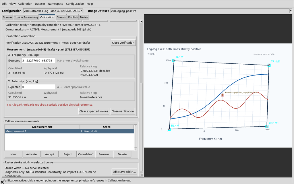
Restoring a positive Expected value makes the comparison available again. Neither the original Dataset nor the calibration corners are removed.
14. A Third Source to Separate the Y Direction from Log Axes
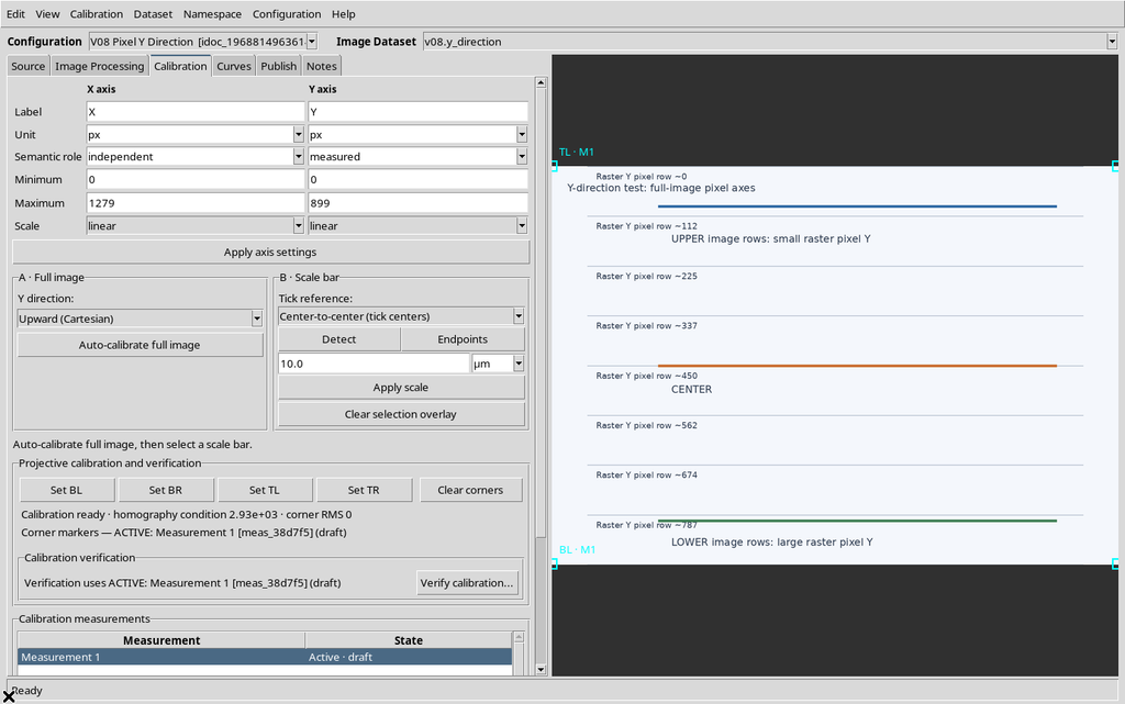
The Calibration tab includes a Y direction control with two entries:
- Upward (Cartesian)
- Downward (image pixels)
This selector is used in the A · Full image → Auto-calibrate full image procedure. On its own it does not change a previous manual log-log calibration.
To avoid confusion between the direction of Y and its logarithmic scale, a third, neutral Dataset was created, with horizontal lines labeled in source pixels.
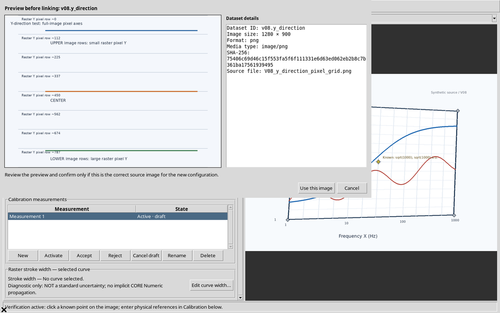
15. Downward (image pixels): Y Increases Downward
In the third configuration, Downward (image pixels) was selected and Auto-calibrate full image was pressed.
For the 1280×900 PNG, the CORE saved the axes X 0–1279 px, Y Minimum 899 px / Maximum 0 px and four corners matching the original raster boundaries.
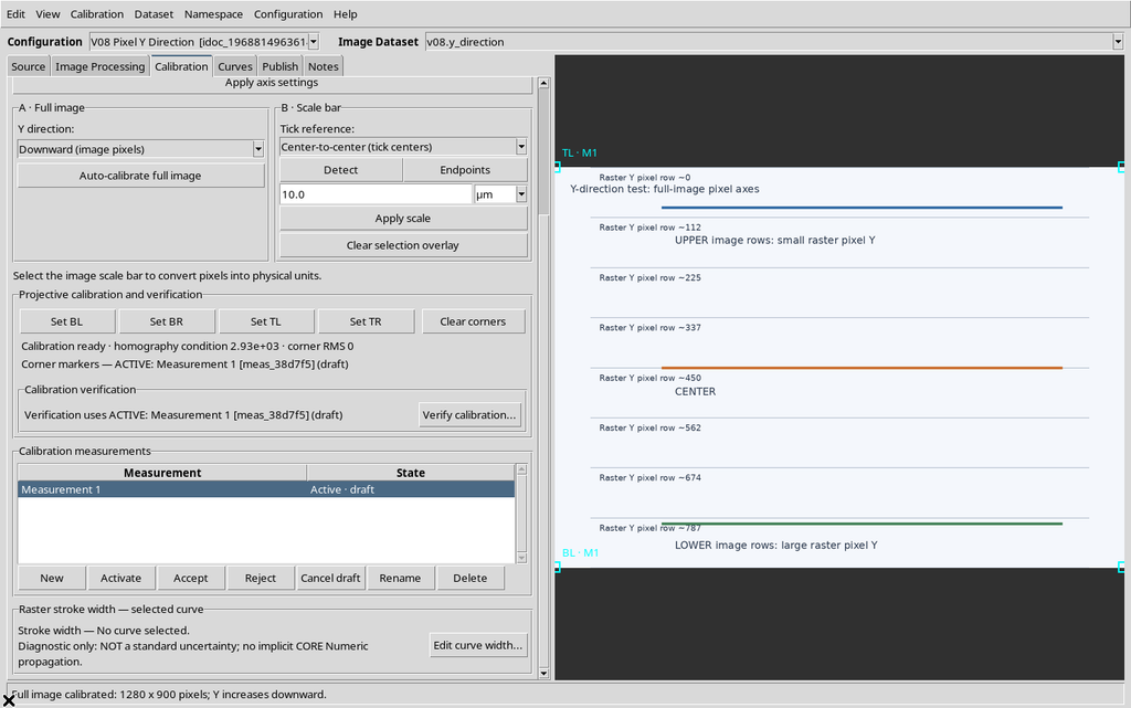
The scale stays linear and the unit px. With this choice the Y of an original pixel is directly its row: for example, pixel 180 has calibrated Y 180 and pixel 700 has calibrated Y 700.
16. Switching to Upward (Cartesian) Requires Confirmation
Selecting Upward (Cartesian) does not automatically replace the calibration that is already valid. Pressing Auto-calibrate full image again, the Viewer showed:
Replace the existing calibration and axis limits with full-image pixel coordinates? Existing digitized points will be recalculated, not deleted.
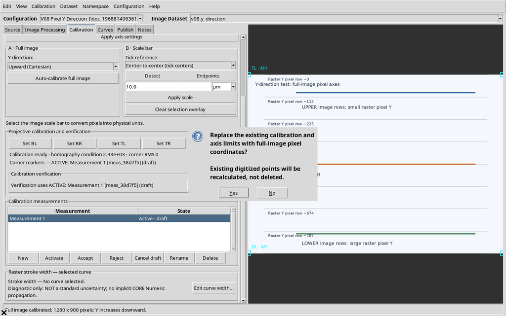
17. Upward (Cartesian): Same Geometry, Inverted Y Numbers
After the new calibration, the Y axis became Minimum 0 px / Maximum 899 px, keeping the same four pixel corners and the same SHA-256 of the source.
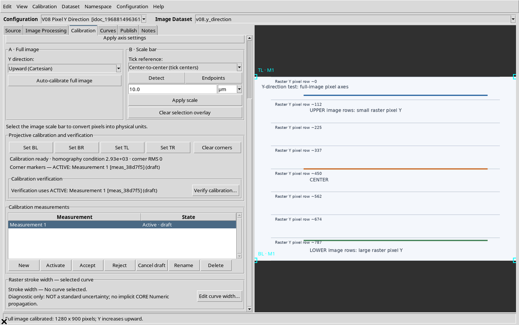
The mathematical comparison on the same raster is:
| Original pixel Y | Downward | Upward |
|---|---|---|
| 180 | 180 px | 719 px |
| 700 | 700 px | 199 px |
For Upward the transformation is Y = (H − 1) − pixel_y, with H=900. The difference concerns the interpretation of the coordinates, not a flip of the PNG pixels.
18. Actual Verification of a Pixel in Cartesian Mode
The Verify calibration… panel was also used for the third configuration. The original click near (500,180) became, after rounding on the canvas, (499.1079; 180.1871) source pixels.
With Expected X = 500 and Expected Y = 719, the Viewer calculated:
Calculated X = 499.1079 px
Calculated Y = 718.8129 px
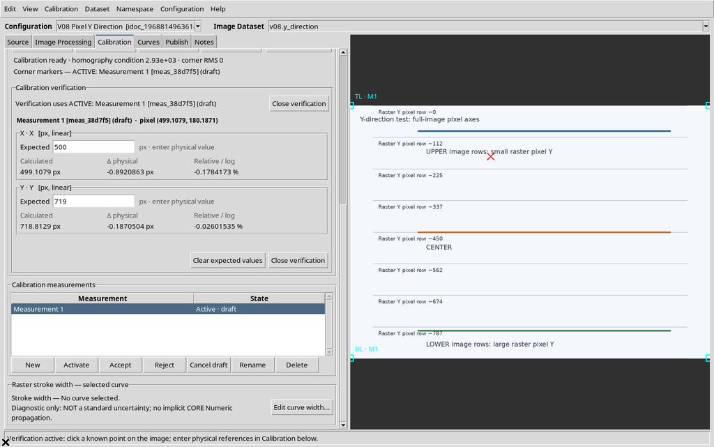
The small deviation is compatible with the discretization of the click. The independent reconstruction confirmed the value. The Y direction of the full-image calibration remains distinct from the Scale = log setting of scientific graphs.
19. Do Not Confuse Direction, Scale and Geometry
The log scale changes the relationship between normalized coordinates and scientific values. Y direction, instead, determines the orientation of the pixel axes when Auto-calibrate full image is used.
A new full-image calibration resets the axes to px, linear: it must not be applied to an already calibrated logarithmic graph in the belief that it only changes the direction of Y. For a manual graph, you need to read the actual physical limits, choose the appropriate mapping and verify known points.
The model can produce corner RMS values close to zero even on a scientifically misinterpreted graph. Always check the semantics of the labels in the image, not just the geometric matrix.
20. Saving and Reopening the Three Configurations
The configurations were saved and reopened through the normal Viewer commands, in the same Session. The CORE returned three separate Workspaces, each linked to its original Image Dataset.
21. Essential Operating Procedure
For an X-log/Y-linear graph, set Scale = log only on X, using positive limits for X; Y stays linear even if it includes zero. For a log-log graph, both limits of both axes must be strictly positive.
After Apply axis settings, click Set BL / Set BR / Set TL / Set TR, check Calibration ready and verify at least one known point with Verify calibration…, distinguishing physical deviations, percentages and decades.
For the vertical direction of the whole raster, select Y direction → Upward/Downward and actually apply Auto-calibrate full image, checking the axes and any replacement confirmation.