

Verifying the Calibration with Known Points and Repeated Realizations
This guide shows how to check a calibration against scientific points independent of those used to build it, interpret logarithmic and linear deviations, repeat the checks for several realizations, and tell temporary diagnostic results apart from the canonical data of the Session.
1. Source: Four Independent Scientific References
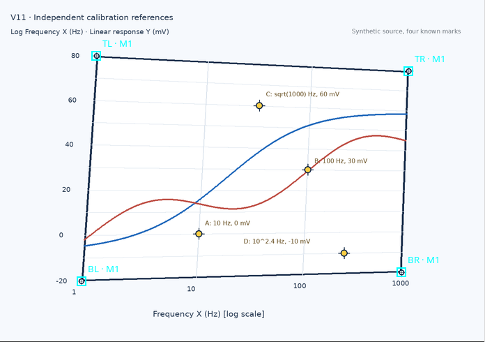
The example uses a synthetic 1280 × 900 pixel PNG, imported as an Image Dataset with the image.raster contract through the GX-TXT Acquisition Handler. The grid is a quadrilateral in slight perspective. The two colored traces are raster pixels, not digitized numerical Datasets.
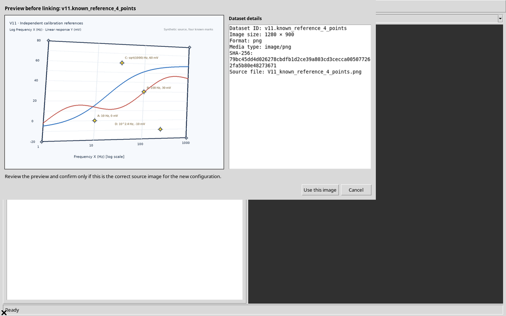
Besides the four calibration targets at the corners, the figure contains four yellow markers A, B, C and D placed at interior points of the graph area. These markers were not used to compute the homography: they are the independent references for the verification.
| Marker | Known X frequency | Known Y response |
|---|---|---|
| A | 10 Hz | 0 mV |
| B | 100 Hz | 30 mV |
| C | √1000 ≈ 31.622777 Hz | 60 mV |
| D | 10^2.4 ≈ 251.188643 Hz | −10 mV |
They are references known by construction of the synthetic figure. They do not represent real instrument calibrations, certified standards or independent repetitions of a physical experiment.
2. Valid Axes and Prerequisites
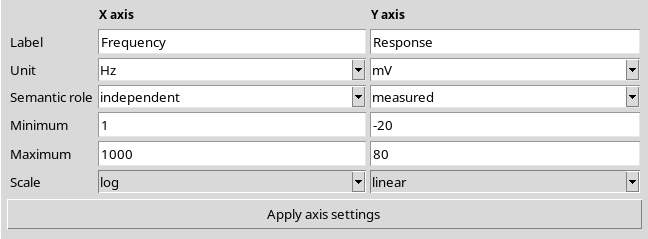
In the Calibration panel, X axis → Frequency, Hz, Minimum 1, Maximum 1000, Scale log and Y axis → Response, mV, Minimum −20, Maximum 80, Scale linear were set. They were applied with Apply axis settings.
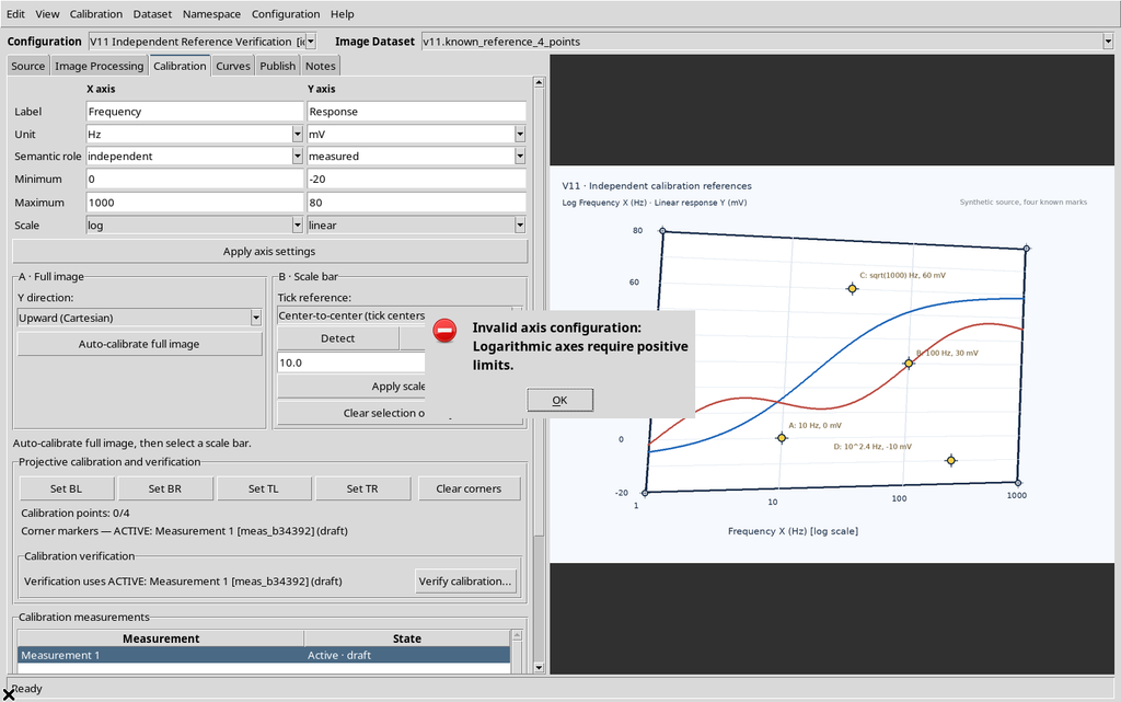
The GUI refuses Verify calibration… if a valid geometric transformation is missing. An attempt at a logarithmic X with Minimum 0 is also rejected: Logarithmic axes require positive limits.
3. First Realization: The Four Geometric Points
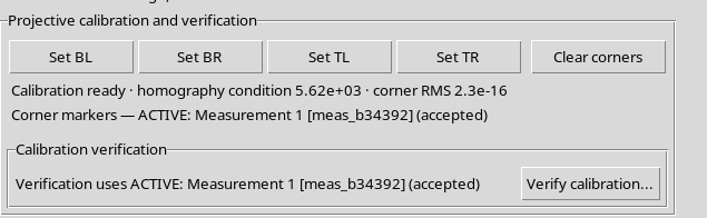
For Measurement 1, the corners of the graph area alone, not the edges of the PNG, were clicked with the Set BL / Set BR / Set TL / Set TR buttons. The Viewer returned Calibration ready and four cyan M1 markers.
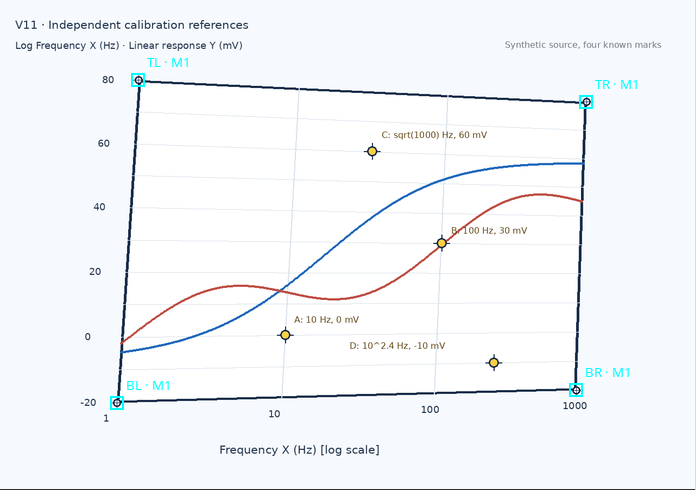
The model uses a four-point homography that transforms the source pixel into the normalized coordinates (u,v). The physical conversion is distinct: the X axis is logarithmic and the Y axis is linear. The initial realization is still in the draft state, even though the geometry is complete; it can be accepted with the Accept command.
4. What the corner RMS Shows, and What It Does Not
The tab showed homography condition ≈ 5.62×10³ and corner RMS ≈ 2.3×10⁻¹⁶ for the first realization.
The small RMS represents the reprojection of the four points used to compute the same homography. It is not proof of the absolute accuracy of the digitization: a transformation exactly constrained by four points can pass through them almost perfectly even when their placement is imprecise.
Markers A–D, not included in the fit, are therefore needed to check the transformation in different areas of the figure. A single verification point is less informative than several distributed points.
5. Opening Verify calibration...: No Invented Values
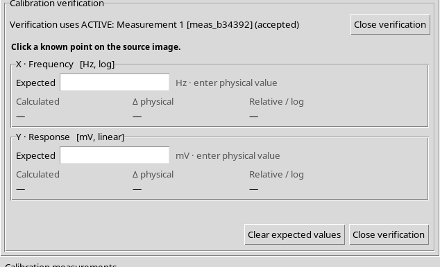
Press Verify calibration… in the Calibration tab. The GUI expands an inline panel, not a second standalone window. Until a known point is clicked on the raster, the panel shows:
Click a known point on the source image.
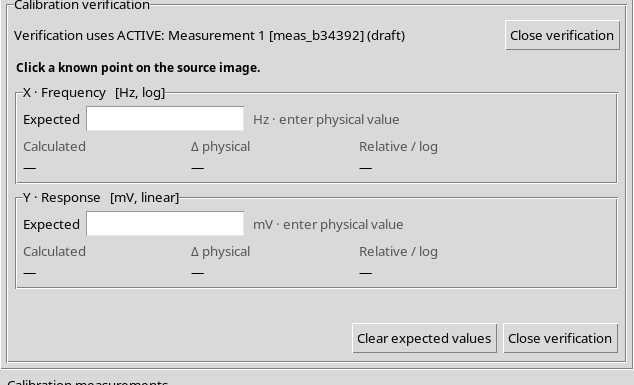
There are Expected fields in physical units and the three result categories Calculated, Δ physical and Relative / log. With no point selected, the results stay —: no measurements are invented.
6. The Red Marker Is a Temporary Diagnostic Choice
During verification, a click on the image places a red diagonal cross at the point used for the transformation. The four calibration corners, drawn in cyan, remain separate.
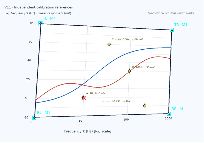
The color and position of the cross come from the Viewer’s actual rendering. It must not be confused with an accepted curve point, with an original target printed in the raster or with a published record.
7. Marker A: Zero Allowed on the Linear Y Axis
On marker A, Expected X = 10 Hz and Expected Y = 0 mV were entered. The GUI reported:
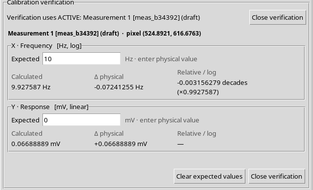
| Axis | Expected | Calculated | Δ physical |
|---|---|---|---|
| X, log | 10 Hz | 9.927587 Hz | −0.07241255 Hz |
| Y, linear | 0 mV | +0.06688889 mV | +0.06688889 mV |
For X, −0.003156279 decades appears, with a multiplicative ratio of about ×0.9927587. For Y, instead, the percentage entry shows —: dividing by a reference Y=0 is undefined, but the physical deviation in mV remains perfectly computable.
Zero is a valid reference on the linear Y axis, not on the logarithmic X axis.
8. Marker B: 10^2 Notation and Decimal Separator
On marker B, Expected X = 10^2, equivalent to the physical value 100 Hz, and Expected Y = 30,0 with a decimal comma were entered. Both formats were accepted by the GUI.
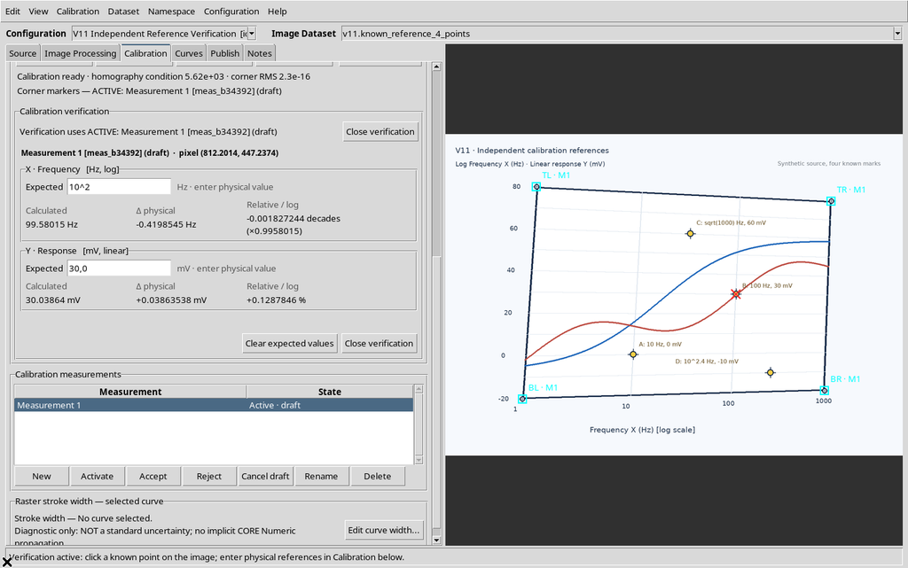
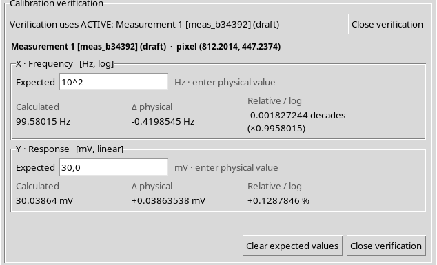
The Viewer displayed 99.58015 Hz and 30.03864 mV, with deviations of −0.001827244 decades on the log X axis and +0.1287846 % on the linear Y axis.
The logarithmic Expected value must be given as the physical value of the quantity, not directly as its logarithm. The 10^2 notation is accepted only because it is explicit; a plain 2 would mean 2 Hz, not 100 Hz.
9. Marker C: 3 Does Not Mean 10³
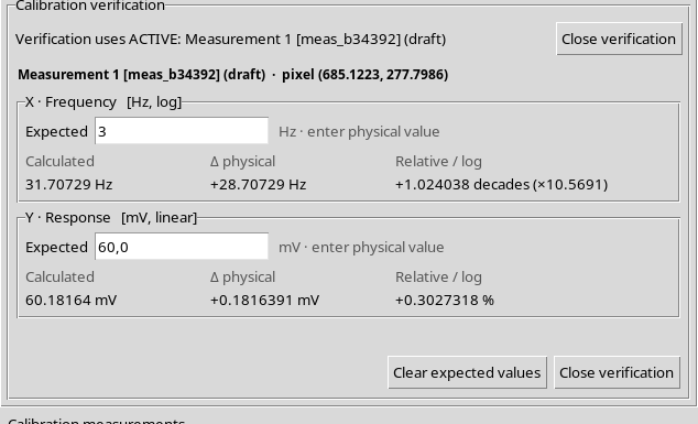
To clarify the difference between a physical value and an exponent, two entries on marker C are compared. Entering X Expected = 3, the Viewer interpreted the number as 3 Hz, not as 10^3 Hz.
Correcting Expected X to 10^1.5 and Y to 60 mV, the panel returned 31.70729 Hz and 60.18164 mV, with +0.001159141 decades and +0.3027318 %.
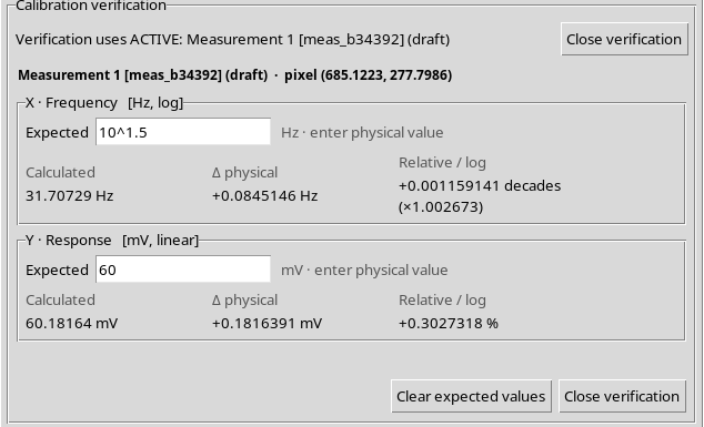
This shows why the expected physical values must be specified clearly. A reference that is numerically valid but refers to the wrong scale can produce a comparison that is mathematically regular and scientifically misleading.
10. Marker D: Negative Linear References
The fourth known point, D, has the references X = 10^2.4 Hz, i.e. about 251.188643 Hz, and Y = −10 mV. The negative Y value is valid, because the axis is linear.
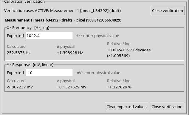
The calculations of the first realization were 252.5876 Hz and −9.867237 mV. The X deviation corresponds to +0.002411977 decades, while the relative Y deviation is +1.327629 %.
The sign of the relative difference is computed by dividing the deviation by the absolute value of the reference, when it is non-zero. There is no need to turn a negative physical quantity into a positive one to validate the linear Expected field.
11. Incorrect Mixed Separator: Invalid Reference
To document a genuinely wrong input, both a comma and a dot were entered in the Expected X field: 1,2.3. The Viewer reported:
Use either a dot or a comma as decimal separator.
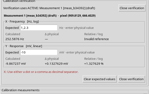
The panel kept showing the calculated X coordinate, but the deviation relative to that reference was marked Invalid reference. This is not a defect of the geometric calibration.
12. Expected X=0 and the Domain of the Log Axis
Entering Expected X = 0 while X is logarithmic, the reference is rejected. The GUI showed:
A logarithmic axis requires a strictly positive physical reference.
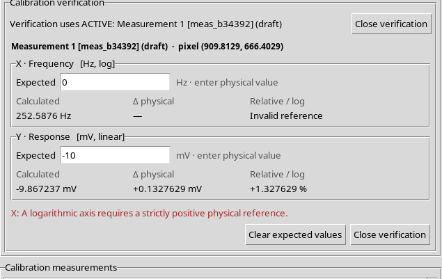
The problem is the domain of the physical reference entered by the operator, not a missing pixel or a change to the matrix. The calculated X value stays visible and is not deleted.
13. A Missing Reference and an Invalid Reference Are Not the Same
Clearing only Expected X, the panel still shows Calculated X but leaves the X deviations without a value: an empty field means no comparison requested.
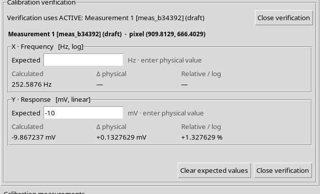
The Expected field for Y can stay filled in and continue to produce its own comparison. An invalid field, instead, produces a specific Invalid reference message. This distinction avoids confusing a check that was not run with a check that failed.
14. Clear expected values Does Not Delete the Verified Point
Pressing Clear expected values, the X and Y fields are emptied at the same time, but the Calculated coordinate of the previously clicked point remains.
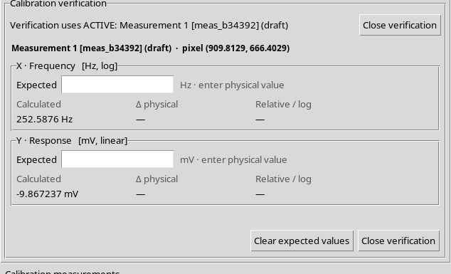
The four corners, the canonical Dataset and the calibration measurement are not changed. The command acts on the temporary references of the comparison, not on the scientific transformation.
15. How the Deviations Are Calculated
The scientific procedure consists of two distinct steps. A homography resolves the source pixel into (u,v); then the physical values are calculated.
For a logarithmic X from 1 to 1000 Hz:
X = 10^(3u) Hz
For a linear Y from −20 to 80 mV:
Y = −20 + 100v mV
The physical deviations are Calculated − Expected. For X, the Relative / log entry uses:
Δlog10(X) = log10(Calculated / Expected) in decades.
For a linear Y, if Expected is non-zero:
Relative ΔY (%) = 100 × (Calculated − Expected) / |Expected|.
If Expected Y=0, the percentage is — and the physical deviation remains available. This is a display rule for the comparison, not an automatic uncertainty propagation procedure.
16. First Realization: Four Observed References
After the four original clicks and the acquisition of references A–D, the scientific results of the first realization are:
| Marker | Calculated X (Hz) | Calculated Y (mV) | Δlog10 X (decades) | ΔY (mV) |
|---|---|---|---|---|
| A | 9.927587 | +0.066889 | −0.003156279 | +0.066889 |
| B | 99.58015 | 30.03864 | −0.001827244 | +0.038635 |
| C | 31.70729 | 60.18164 | +0.001159141 | +0.181639 |
| D | 252.5876 | −9.867237 | +0.002411977 | +0.132763 |
17. Distribution of the Checks and Quality of the References
The four markers are spread over different areas of the image. The quality of the verification does not depend only on the size of a residual, but also on the quality of the chosen references, on the unambiguous identification of the target and on the spatial coverage of the graph.
The mean of the absolute values of the observed deviations, purely descriptive, was in the first realization:
- X: 0.00213866 decades;
- Y: 0.104982 mV.
These are not standard uncertainties: they are arithmetic summaries of four verification errors on a single synthetic raster. They are not estimates of instrumental error, confidence intervals or accuracy certifications. The small corner RMS does not replace these independent checks.
18. The Verification Closes When You Change Tab
If, while Verify calibration… is active, you select the Curves tab, the inline panel is closed automatically. Back in Calibration, the button again shows Verify calibration… and the temporary cross does not stay active.
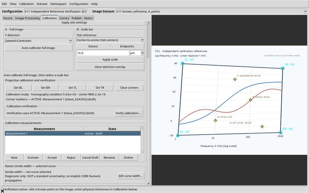
The Workspace kept the axes and all four corners. Verification is an operating mode and does not insert a point into the list of curves.
19. Accepting the First Measurement and Creating a Second Realization
The first complete calibration was classified accepted with the Accept command of the Calibration measurements panel.
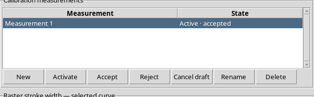
Pressing New, the Viewer generated Measurement 2, initially draft and with zero corners; the homography of Measurement 1 remained stored and accepted.
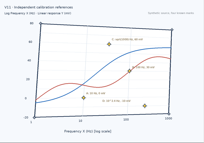
The second realization uses the same original Dataset with identical logarithmic X and linear Y. It is therefore not a second physical experiment: it is a new pointing of the four corners on the same figure.
20. Second Four-Corner Calibration
The four M2 corners were clicked again with small intentional shifts compared with M1. The Viewer built a second homography, distinct but complete. It was then accepted with Accept.
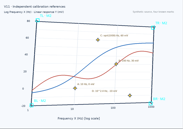
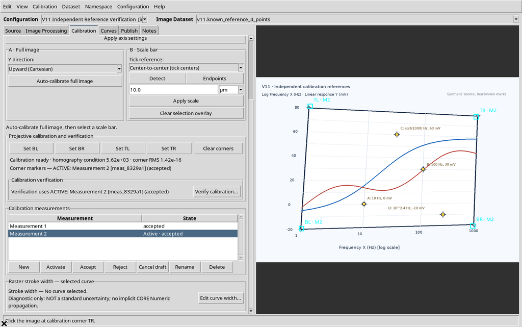
The group now has two accepted measurements with different permanent identifiers and four geometric points each. The source raster was not replaced and its SHA-256 stayed unchanged.
21. Selected Does Not Mean ACTIVE
The Measurement 1 row was selected while Measurement 2 remained active. The panel reported Corner markers — ACTIVE: Measurement 2.
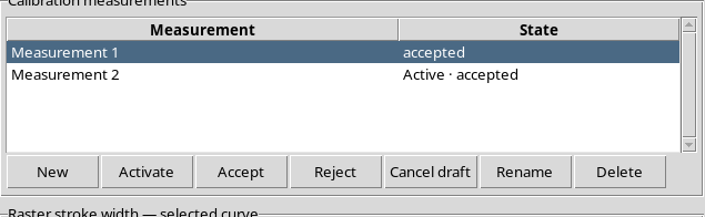
The result of Verify calibration…, run on marker B, also explicitly identified Measurement 2 (accepted), not the merely highlighted measurement.
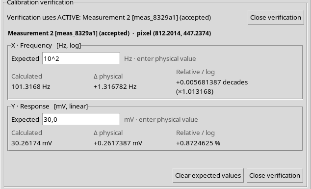
To compare different realizations you must press Activate on the desired measurement. Without activating it, the Viewer keeps interpreting the pixels according to the transformation already active.
22. Second Measurement: The Same Four Scientific Markers
Markers A–D were clicked again on the same raster, at identical canvas coordinates to the first realization. The only difference is the calibration applied.
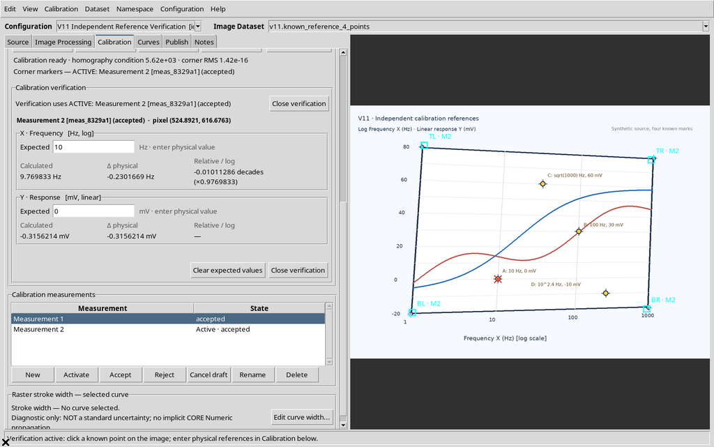
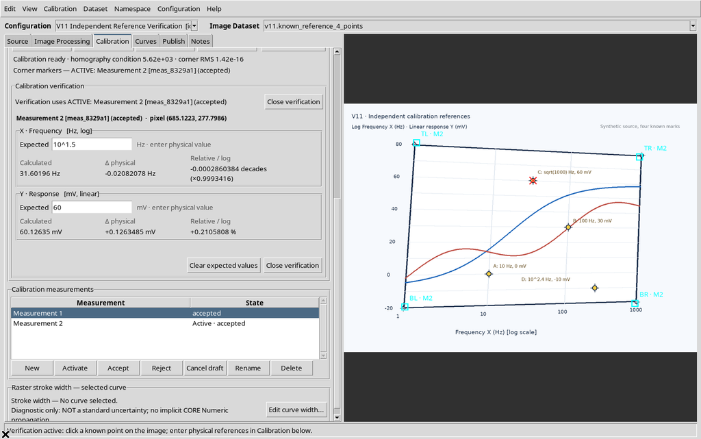
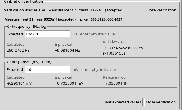
The readouts of the second accepted measurement are:
| Marker | Calculated X (Hz) | Calculated Y (mV) | Δlog10 X (decades) | ΔY (mV) |
|---|---|---|---|---|
| A | 9.769833 | −0.315621 | −0.01011286 | −0.315621 |
| B | 101.3168 | 30.26174 | +0.005681387 | +0.261739 |
| C | 31.60196 | 60.12635 | −0.000286038 | +0.126349 |
| D | 260.2702 | −9.296161 | +0.01542452 | +0.703839 |
23. Comparing Realizations: Description, Not Uncertainty
Comparing the same four known points, the maximum absolute X residual observed goes from about 0.00315628 decades in M1 to 0.01542452 decades in M2. The maximum absolute Y deviation goes from about 0.181639 mV to 0.703839 mV.
The descriptive mean of the absolute deviations in the second realization is 0.00787620 decades for X and 0.351887 mV for Y.
These values allow a consistency comparison against the known references of the synthetic figure, but they do not justify claiming instrumental precision, random error or covariance. The realizations are not independent physical data and are also affected by the quantization of the click in the viewport.
Both corner RMS values are almost zero (of the order of 10⁻¹⁶), because they measure the reprojection of the same four corners used in the calculation; this does not prevent marker D of M2 from having a larger independent deviation.
24. Reactivating the First Measurement and Checking Software Repeatability
With Measurement 1 selected, Activate was pressed. The Viewer closed the temporary M2 verification and restored the first transformation.
Repeating the click on marker B, the GUI again returned 99.58015 Hz and 30.03864 mV, identical to the values observed before acceptance and before the M1→M2→M1 switch.
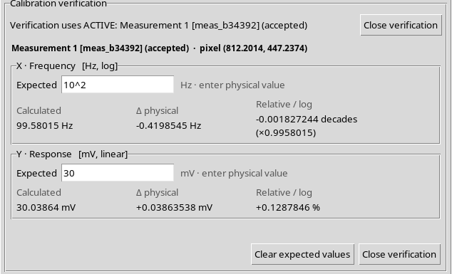
This is a check of the repeatability of the software calculation on an identical canvas event and identical geometric points, not of the repeatability of a laboratory measurement.
25. Esc Removes the Cross, Not the Calibration Data
The red cross of the known point is drawn as a transient canvas overlay. In verification mode, the Viewer created two red diagonal segments.
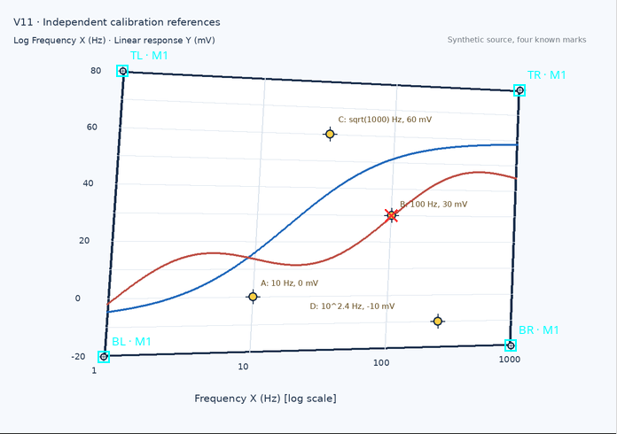
Pressing Esc, the GUI closed the verification, removed these segments and returned the button to Verify calibration….
The original markers A–D remained in the raster and the four cyan calibration markers stayed visible: no geometry of the accepted measurement was deleted.
26. Save, Close and Reopen: What Is Kept
The Viewer was saved with Configuration → Save configuration, closed with the normal window protocol and reopened through Viewers → Digitalizer in the same Session.
What was restored: a single Image Dataset, two accepted measurements, the same IDs, the scientific axes, the two homographies and the first measurement as active.
The verification, instead, was empty again: no control cross and the Expected fields initially without values, even though typed references were still present before saving.
The verification is temporary: the results for markers A–D are not stored automatically in the canonical calibration and do not constitute a metrological certification.
27. Quality Schema, Preview and Canonical Content: A Necessary Distinction
The Quality Schema v2 for curves is produced when numerical Datasets are published. In this example no curves are digitized and no numerical tables are published.
The results of Verify calibration… belong to the Viewer’s temporary diagnostics and must not be described as a persistent statistic in Calibration & Quality of the Dataset Preview. The Dataset Preview tabs and the plots produced through Plot Dataset refer to numerical Datasets actually published, not to these temporary verifications.
The distinction between calibration corners, accepted measurements, known verification points and published series points is substantial. A known verification point is not automatically added to a curve and does not provide a standard uncertainty.
28. Short Operating Procedure
Prepare a Digitizer Configuration with a defined source and physical axes; calibrate the four corners with Set BL/BR/TL/TR. After Calibration ready, press Verify calibration…, click one or more independent known points and enter the Expected values in their physical units.
For logarithmic axes, the Expected values must be positive and can be written as 100, 1e2 or 10^2; do not enter 2 meaning 10^2 implicitly. On linear axes zero and negative values are allowed, but the percentage with an Expected value of zero is undefined.
Verify points spread across the image, not only near the corners. With several calibration measurements, check ACTIVE and use Activate before comparing the same points. The observed deviations help to detect calibration errors, but they are not automatically instrumental uncertainties.