

Dataset Preview — Reading Calibration & Quality
The Calibration & Quality tab of the Dataset Preview gathers information about the calibration and the quality checks published together with the scientific curves of the Curve Digitalizer. It lets you check source identity, units, accepted calibrations, data consistency and raster diagnostics without modifying the Dataset.
The example uses a synthetic graph with three manually digitized curves, each with eight points, on a raster of 1280 × 900 pixels. The published Dataset contains 24 rows and a single accepted calibration. The quality indicators describe software checks and raster characteristics: they are not automatically equivalent to a metrological evaluation of accuracy or uncertainty.
1. Two Tools with Different Tasks
The Curve Digitalizer Calibration tab serves to set up and accept the transformation from pixel coordinates to scientific coordinates. Calibration & Quality, instead, belongs to the Dataset Preview: it shows the results and the information recorded by the publication.
There is no need to return to the Viewer to read these metadata. Do not use the Preview tab as if it were a command to correct a calibration: the information shown is intended for consultation.
2. Completing the Calibration in the Curve Digitalizer
The example starts from the definition of the axes Elapsed time (s) and Detector response (mV), both linear, with X from 0 to 10 s and Y from −20 to 80 mV. The calibration requires the four references BL, BR, TL and TR and is accepted in the Viewer.
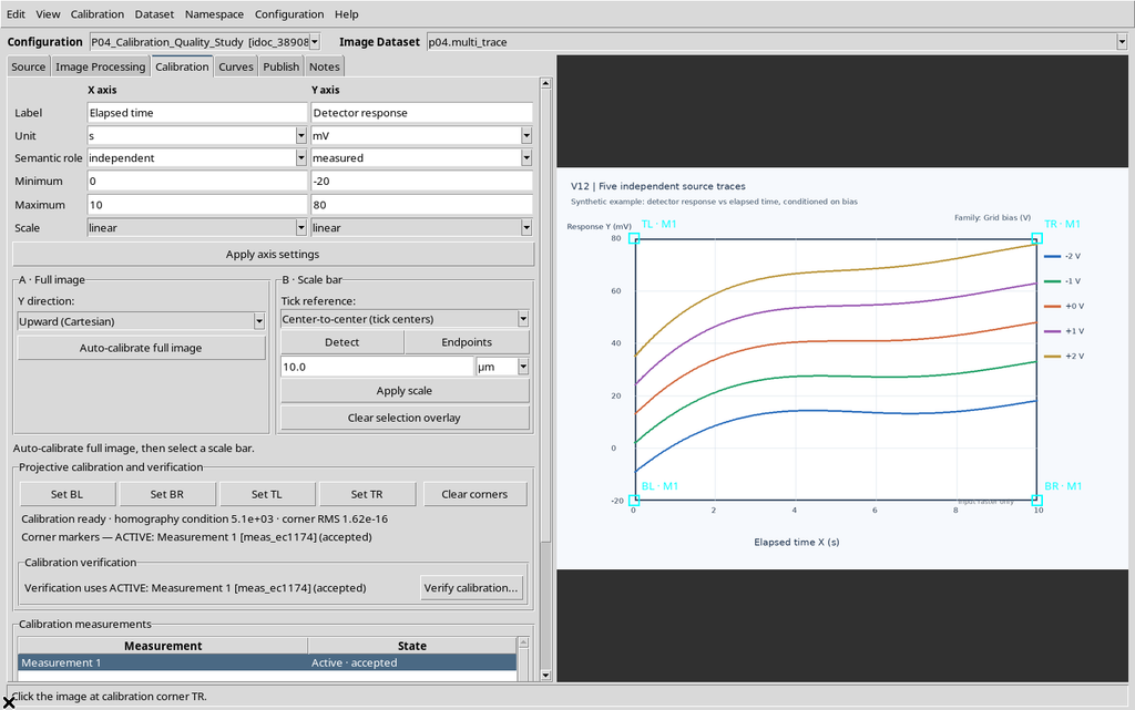
Acceptance describes the completion of the procedure in the software. It does not in itself constitute an independent verification with external experimental references.
3. Preparing Three Curves with Their Points
Three independent curves were created, Bias -2 V, Bias -1 V and Bias +0 V, with eight manual points per curve. The two further lines in the raster graph remained simple elements of the image.
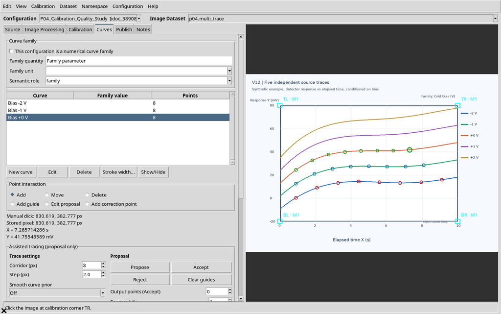
Knowing the number of curves and points is important in order to compare it with the counts displayed later in the Quality tab.
4. Choosing a Realization to Publish
In the Publish tab the Viewer presents the accepted calibration realization and the planned scientific output. The example uses separate, that is, a Dataset corresponding to a single selected realization.
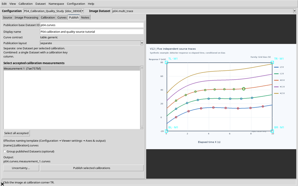
This choice will be reported in the metadata as Calibration mode: separate, distinct from other possible publishing modes.
5. Publishing the Dataset Before Consulting Quality
Press Publish selected calibrations and check that the publication has been registered. The Quality information is not an analysis to be built by reading the image directly: it accompanies the canonical Dataset produced by the Viewer.
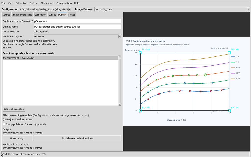
The published output does not replace the raster source or the editable document in the Viewer.
6. Opening the Correct Dataset in the Framework
In the main window choose Dataset → Preview and select the numerical Dataset, not the previous Image Dataset. In the example the result has the table.generic contract and presents the framework’s scientific consultation tabs.
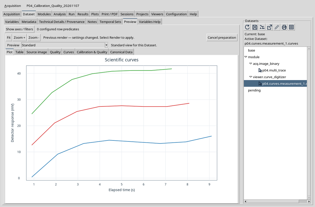
The identifier displayed belongs to the exercise Session. In a different project always use the actual identity of the published Dataset.
7. Opening Calibration & Quality
In the row of tabs choose Calibration & Quality. The panel presents a text consultation with the PREVIEW METADATA section and various field-value pairs. It is not the digitizing Canvas and contains no buttons to accept or move points.
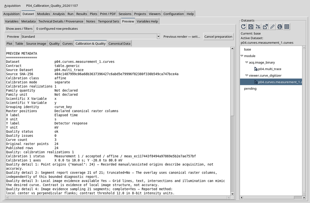
To read all the information, use the panel’s vertical scroll bar. Some diagnostics are longer than the visible portion.
8. Reading Dataset, Contract and Source Dataset
The first fields indicate Dataset, Contract and Source Dataset. They distinguish the numerical result, the type of representation and the image from which the point positions were derived.
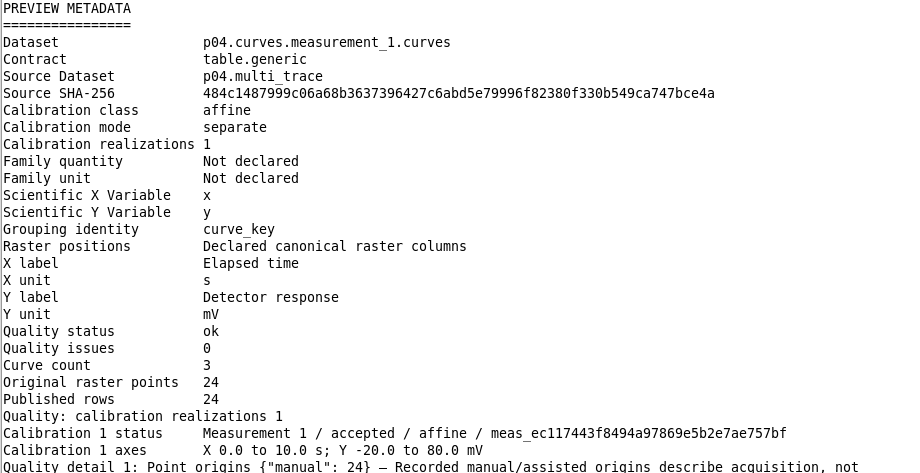
The scientific Dataset of the example is distinct from the source raster. Their association is kept in the provenance, not in the position of the windows on the screen.
9. Understanding Source SHA-256
Source SHA-256 is the digital fingerprint recorded for the original image. The value serves to identify the source exactly, even when two files have the same name or the same dimensions.
In the documented case the source check returns verified. The identity of the image must not be replaced with a visually similar preview: the colour of a line is not proof of provenance.
The Source SHA-256 field shows the digital fingerprint associated with the image used for digitization. When the Dataset is consulted later, this reference helps distinguish the exact origin of the pixels from other images with similar names or appearance.
Source verification concerns the consistency of the raster identity. It does not prove the correctness of the units, the accuracy of the calibration or the absence of experimental uncertainties. For this reason the Source SHA-256 field must be interpreted together with the other states of the Quality report.
10. Calibration Class and Calibration Mode
The panel shows Calibration class: affine and Calibration mode: separate. The first field describes the declared class of the transformation, the second the mode in which the realization was published.
Do not confuse these values with the characteristics of the graph: a declared transformation and a successful publication do not provide an estimate of the physical uncertainty of the measurement.
11. Calibration Realizations Does Not Mean Experimental Replicates
Calibration realizations: 1 indicates a single published calibration realization. It is the number of configurations available in the result, not the number of repeated instrumental trials.
If only one realization has been registered, a statistical dispersion between calibrations cannot be derived automatically. Do not assign zero uncertainty to a dispersion that cannot be calculated.
12. Recognizing the Scientific Variables and Units
The Scientific X Variable and Scientific Y Variable fields identify the columns of the Dataset. Their labels are Elapsed time, in s, and Detector response, in mV.
The recorded units come from the calibration and publishing work. They do not represent information inferred from the Plot magnification or from the raster dimensions.
13. Family Quantity, Family Unit and Grouping Identity
In the example Family quantity and Family unit are Not declared because the three curves were published as independent series and not as a parameterized numerical family. This is not an error.
Grouping identity: curve_key indicates the column used to distinguish the curves stably. The readable names of the series help the user, but the canonical identifiers remain the reference for associating their points.
14. Quality Status and Quality Issues
The publication shows Quality status: ok and Quality issues: 0. This means that the report did not record problems in the check categories provided for this Dataset.
These two fields do not mean that the image was measured with known accuracy. The diagnostics of the acquisition, the geometry and the raster must be interpreted within their declared scope.
15. Curve Count, Original Raster Points and Published Rows
The values are Curve count: 3, Original raster points: 24 and Published rows: 24. They are consistent with the three eight-point curves created in the Viewer.
This agreement documents that the original points were represented in the publication without an unexpected change in the count. It is not a quantitative verification of the error in abscissa or ordinate.
16. Reading Calibration 1 Status and Its Axes
The tab describes Calibration 1 status as Measurement 1 / accepted / affine and reports the internal identifier of the realization. Its axes are X 0.0 to 10.0 s; Y -20.0 to 80.0 mV.
The axis labels and the fact that the realization is accepted can be checked directly by comparing the tab with the work carried out in the Viewer.
17. The Diagnostics Start from the Origin of the Points
Scrolling the panel, the Quality detail entries appear. The first describes Point origins: in the example 24 manual were recorded, that is, 24 manually acquired points.
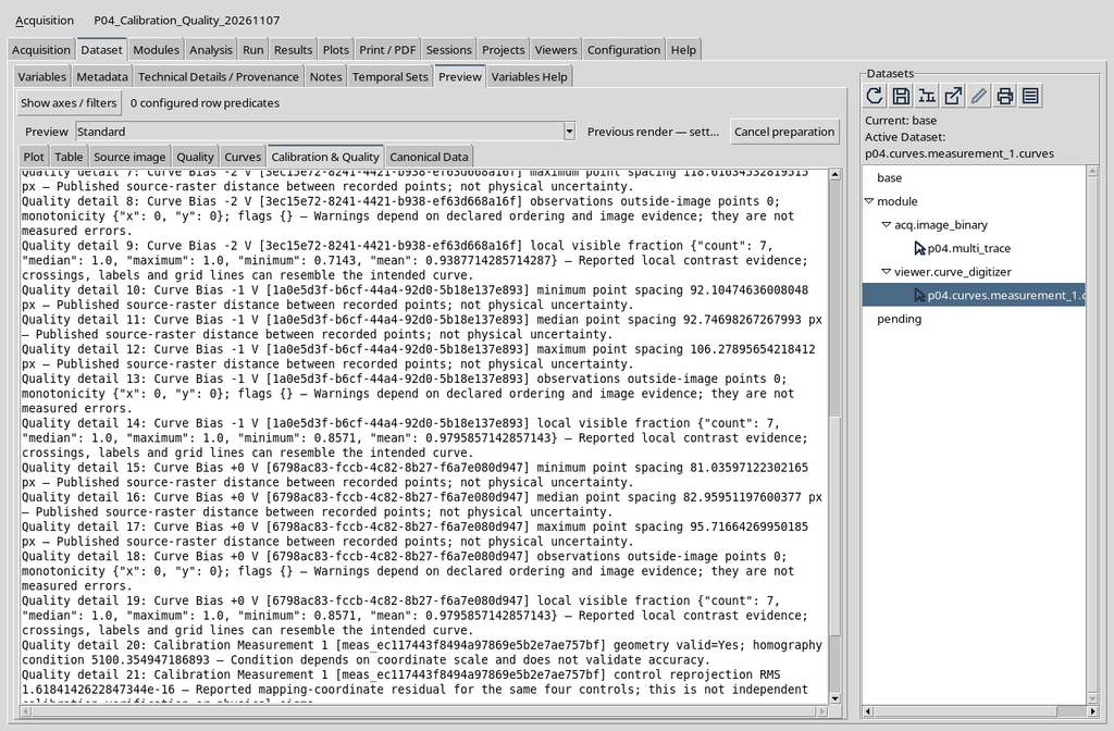
The manual or assisted origin documents the acquisition procedure. It does not, on its own, constitute an estimate of the metrological quality of the tracing.
18. Segment Report Coverage and Number of Segments
A curve with eight consecutive points normally produces seven segments between adjacent pairs. Three curves of this type therefore generate 21 segments; the report indicates 21 of 21; truncated=No.
The value describes the coverage of the check on the published segments. It must not be interpreted as 21 new independent experimental observations.
19. Local Image Evidence: Evidence from the Raster
The report shows Local image evidence available: Yes. For the example, 21 segments were examined with the method indicated as local_center_vs_perpendicular_flanks, using a contrast threshold of 12.0 in 8-bit intensity units.
This is a check on the local structure of the image: grids, crossings, labels and contrast can mimic a curve. Contrast evidence is not equivalent to physical accuracy.
20. Distinguishing Pixel Spacing from Physical Uncertainty
For each curve, minimum, median and maximum distance values between consecutive points are available, expressed in px. The report indicates, for example, for the Bias -2 V curve a minimum distance of about 105.04 px and a maximum of about 118.62 px.
These distances describe the geometric sampling of the points in the raster. They are not standard uncertainties in seconds or millivolts and cannot be used directly as error bars.
21. Local Visible Fraction and the Limits of Contrast
Another indicator is local visible fraction, calculated on the image samples used for the segments. In the example some fractions are below 1 even though no general quality problem was reported.
The fraction does not measure the probability that the curve is scientifically correct. It serves to describe how much of the local signal shows the image evidence expected by the check.
22. Valid Geometry and Conditioning
Towards the bottom of the panel Calibration Measurement 1 geometry valid=Yes appears, with a homography condition value of around 5100.35. The condition depends on the scale of the coordinates and is a numerical-geometric indicator.
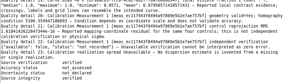
Do not use the condition number as a direct evaluation of the precision of the instrument or of the absolute goodness of the calibration.
23. Control Reprojection RMS Is Not Independent Accuracy
The GUI reports a control reprojection RMS of about 1.62 × 10⁻¹⁶ for the same four references used in the transformation. The value is very small because it refers to the reprojection of the controls used to determine the calibration.
It is not a verification with independent points and must not be interpreted as zero physical uncertainty. An almost zero numerical residual can coexist with errors in the choice of the original references.
24. Independent Verification: Not Recorded
The report indicates independent verification: available=false; status=not_recorded. Results of a verification distinct from the four calibration controls are therefore not available.
The absence of verification must be reported as such: it does not authorize declaring that the experimental error is zero. Similarly, a single realization does not automatically provide a dispersion between calibrations.
25. The Three Final States Are Not Equivalent
At the end of Calibration & Quality you can read Source verification: verified, Accuracy status: not_assessed and Uncertainty status: not_declared.
[IMAGE 10] — 12_native_Quality_accuracy_uncertainty_status_bottom.png
Figure 10. Bottom of the tab with information on the geometry, independent verification not recorded and final states.
The verified identity of the source confirms the consistency of the declared link within the scope of the available checks. It does not certify the physical measurement; accuracy remains not assessed and an undeclared uncertainty cannot be replaced with zero.
26. Ordinary Quality and Calibration & Quality
In addition to the additional Calibration & Quality tab, the CORE Preview presents a Quality tab. The latter organizes the same published information in rows with the columns Diagnostic, Value, Unit and Meaning.
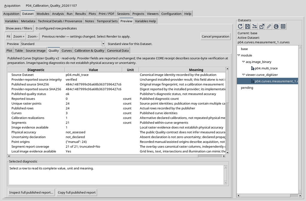
The additional view makes compact reading of the calibration metadata easier; the Quality table helps consult the meaning associated with the individual indicators.
27. The Unit and Meaning Columns Avoid Wrong Interpretations
In the Quality tab, the Unit column makes it possible to distinguish counts from distances in pixels, while Meaning explains the scope of the value. The presence of a numerical value does not imply that it is a measured physical quantity.
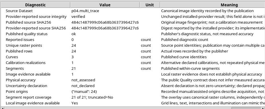
The interface distinguishes the description of the check method from its result: read both before reporting a conclusion in the scientific documentation.
28. Selecting Physical Accuracy
In the Quality table click the Physical accuracy row. The lower Selected diagnostic panel shows the value not_assessed and specifies that the Quality contract does not automatically infer a measured accuracy.
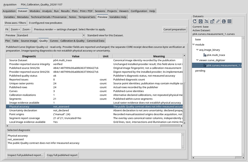
Selecting a row does not change the Dataset. It is an operation for consulting details already recorded.
29. Selecting Uncertainty Declaration
Click Uncertainty declaration. The value is not_declared: it means that an uncertainty declaration is not available in the publication.
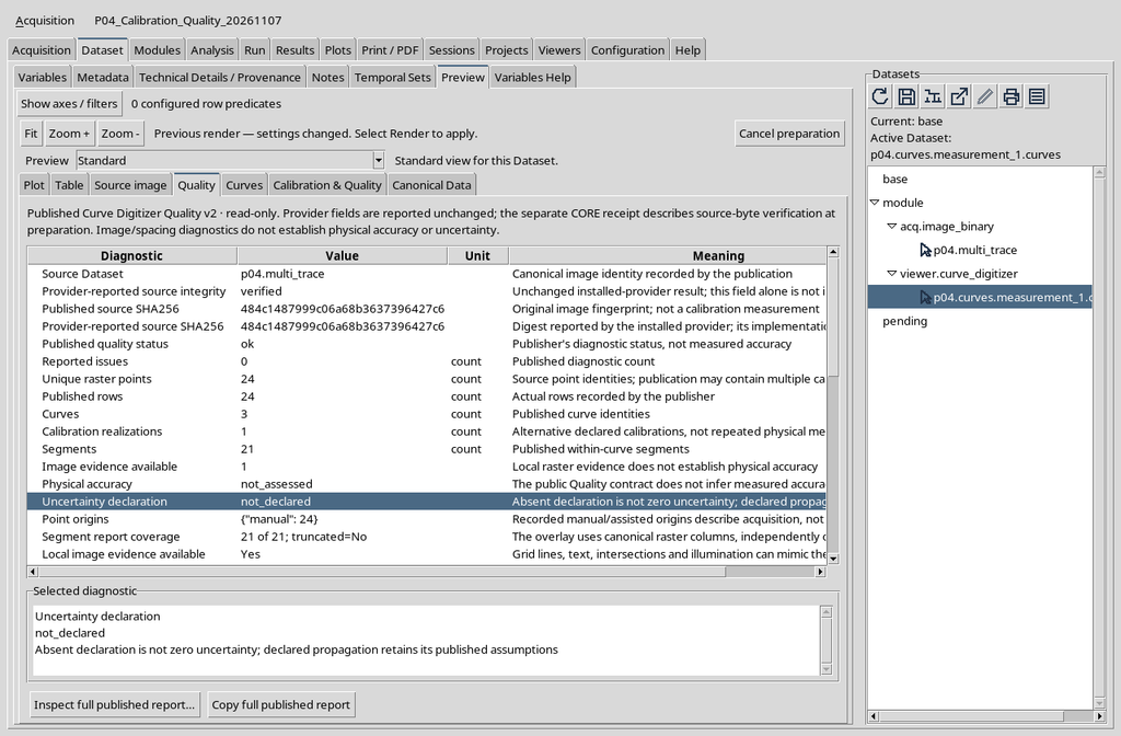
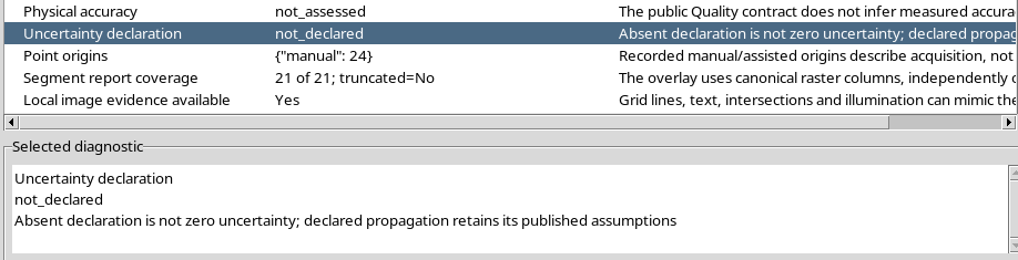
If physical uncertainties are needed, they must be provided through a model or a documented procedure and published consistently. Do not derive them arbitrarily from the line width or from the control RMS alone.
30. Verifying the Source Provenance
The Provider-reported source integrity row shows verified. The description specifies that the provider’s result must not be confused, on its own, with an independent and complete verification of the bytes by the CORE.
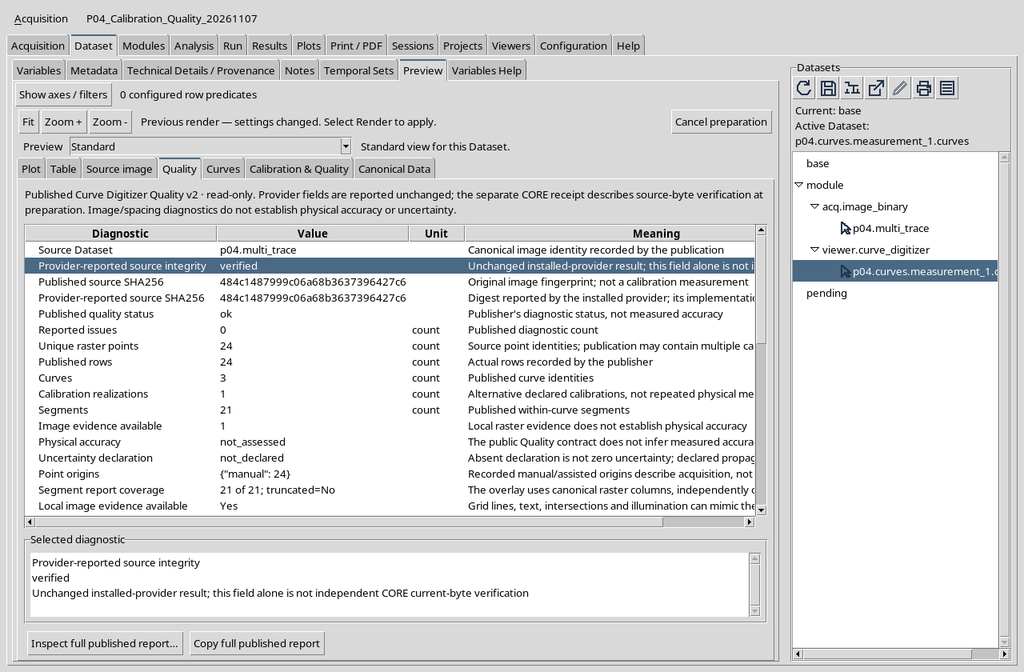
The SHA-256 recorded for the original raster must be considered together with the information on the Session and on the provenance of the publication.
31. Reading Reported Issues
The Reported issues row is 0 count. It expresses the number of problems published by the diagnostics system for this Dataset and for the rules applied.
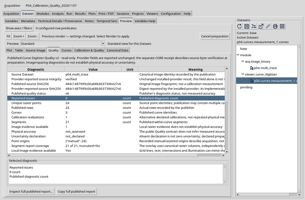
A correct description in the report is “no diagnostic problem reported”, not “experimentally perfect curve”.
32. Returning to the Calibration & Quality Tab
After consulting the ordinary table you can return to the Calibration & Quality tab to find the calibration summary and the entire text list again. Switching between the two tabs does not require a new publication.
The scrolling, navigation and diagnostic selection operations modified neither the raster source nor the canonical content of the published Dataset.
Returning from Quality to Calibration & Quality you find the same panel already illustrated at the start: there is no need to reproduce a second screenshot of it. Check that the Dataset identifier has not changed and that the calibration information always refers to the same publication.
Switching between the two views does not repeat Publish, does not generate a new report and does not automatically correct scientific data. The three states Source verification, Accuracy status and Uncertainty status must be reread separately.
33. The Full Quality Report and the Summary Information
The CORE table also exposes the buttons Inspect full published report… and Copy full published report. They are commands to examine or copy the published diagnostic report in depth, not to change the accepted calibration.
The publication in the case illustrated contains a Quality Report v2, with data on curves, segments, local evidence and calibration. The full report is richer than the summary visible at the top of the tab.
34. Checking Consistency Before Using the Data
Before citing a result, check the selected Dataset, the source ID, the X/Y units, the number of realizations and the number of points. Check Quality status, Source verification, Accuracy status and Uncertainty status separately.
A value can be available, consistent and published without its physical accuracy having been assessed. The meaning of each state must remain distinct.
35. Summary of the Scientific Reading
The operating sequence is: Dataset → Preview → select the numerical Dataset → Calibration & Quality. Scroll through the information down to the calibration details and the three final states; to interpret the individual indicators also use the CORE Quality tab.
In the example there are one accepted calibration, three curves, 24 manual points, 21 segments and no diagnostic report. The source is verified, but physical accuracy and uncertainty are not declared as assessed. It is this distinction that makes reading the Quality report useful for scientific work.